DANL 200: Introduction to Data Analytics
DANL 200 - Lecture 15 Class Exercises -
Answers
Byeong-Hak Choe
2023-02-14
Loading R packages for Class Exercises
library(tidyverse)Tweets with #climatechange
The following data is for Class Exercises:
NY_CC_tweets <- read_csv(
  'https://bcdanl.github.io/data/NY_tweets_cc_no_contents.csv')
Variable Description
id_user: a unique identification number for a Twitter user whom retweeted to a tweet with #climatechange or #globalwarming.id_city: a unique identification number for a city.FIPS: a unique identification number for a county.
Each row represents an observation of a retweet to a tweet with #climatechange or #globalwarming.
Each row includes a Twitter user’s geographic information at city or
county levels (variables FIPS, county,
city) as well as information about timing when a Twitter
user retweeted (variables year, month,
day, hour, minute,
second).
Q1a
How many Twitter users retweeted on the date, January 1, 2017?
# 1. using filter(), select(), and distinct()
Q1a <- NY_CC_tweets %>%
  filter(year == 2017, month == 1, day == 1) %>%
  select(id_user) %>%
  distinct()
# 19


# 2. using filter() and summarise() with n_distinct()
Q1a <- NY_CC_tweets %>%
  filter(year == 2017, month == 1, day == 1) %>%
  summarise(n_users = n_distinct(id_user))
# 19


# 3. using filter(), select() and mutate() with n() and distinct()
Q1a <- NY_CC_tweets %>%
  filter(year == 2017, month == 1, day == 1) %>%
  select(id_user, year, month, day) %>%
  distinct() %>%
  mutate( n_users = n() ) %>%
  select( year, month, day, n_users ) %>%
  distinct()
# 19
Q1b
Which city is with the third highest number of retweets on the date, December 1, 2017?
# 1. filter(), group_by(),
# mutate() with n(), select(), distinct(), and arrange()
Q1b <- NY_CC_tweets %>%
  filter(year == 2017, month == 12, day == 1) %>%
  group_by(id_city) %>%
  mutate(n_rt = n()) %>%
  select(id_city, city, n_rt) %>%
  distinct() %>%
  arrange(-n_rt)
# brooklyn, ny


# 2. filter(), group_by(),
# summarise() with n(), and arrange()
Q1b <- NY_CC_tweets %>%
  filter(year == 2017, month == 12, day == 1) %>%
  group_by(id_city, city) %>%
  summarize(n_rt = n()) %>%
  arrange(-n_rt)
# brooklyn, ny


# 3. filter(), group_by(),
# summarise() with n(), ungroup(), and mutate() with dense_rank()
Q1b <- NY_CC_tweets %>%
  filter(year == 2017, month == 12, day == 1) %>%
  group_by(id_city, city) %>%
  summarize(n_rt = n()) %>%
  ungroup() %>%  # dense_rank() calculates rankings within a group.
  mutate(ranking = dense_rank(desc(n_rt))) %>%
  filter(ranking == 3)
# brooklyn, ny
Q1c
For each year, find the top 5 Twitter users in NY state in terms of the number of retweets they made in NY state. In which city and county do these users live in?
# 1. group_by(), mutate() with n(),
# group_by(), mutate() with dense_rank(),
# filter(), select(), distinct(), and arrange()
Q1c <- NY_CC_tweets %>%
  group_by( id_user, year ) %>%
  mutate( n_rt = n() ) %>% # the number of retweets for each user for each year
  group_by( year ) %>%  # dense_rank() calculates rankings within a group.
  mutate( n_rt_rank = dense_rank( desc(n_rt) ) ) %>%
  filter( n_rt_rank <= 5 ) %>%
  select(-(month:second)) %>% # Need to remove from 'month' to 'second' to use distinct().
  distinct() %>%
  arrange(year, n_rt_rank)


# 2. group_by(), summarise() with n(),
# filter(), arrange(), and head()
Q1c_2012 <- NY_CC_tweets %>%
  group_by( id_user, year, city, county ) %>%
  summarise( n_rt = n() ) %>%
  filter( year == 2012 ) %>%
  arrange(-n_rt) %>%
  head(5)

Q1c_2013 <- NY_CC_tweets %>%
  group_by( id_user, year, city, county ) %>%
  summarise( n_rt = n() ) %>%
  filter( year == 2013 ) %>%
  arrange(-n_rt) %>%
  head(5)

Q1c_2014 <- NY_CC_tweets %>%
  group_by( id_user, year, city, county ) %>%
  summarise( n_rt = n() ) %>%
  filter( year == 2014 ) %>%
  arrange(-n_rt) %>%
  head(5)

Q1c_2015 <- NY_CC_tweets %>%
  group_by( id_user, year, city, county ) %>%
  summarise( n_rt = n() ) %>%
  filter( year == 2015 ) %>%
  arrange(-n_rt) %>%
  head(5)

Q1c_2016 <- NY_CC_tweets %>%
  group_by( id_user, year, city, county ) %>%
  summarise( n_rt = n() ) %>%
  filter( year == 2016 ) %>%
  arrange(-n_rt) %>%
  head(5)

Q1c_2017 <- NY_CC_tweets %>%
  group_by( id_user, year, city, county ) %>%
  summarise( n_rt = n() ) %>%
  filter( year == 2017 ) %>%
  arrange(-n_rt) %>%
  head(5)


# 4. group_by(), mutate() with n(),
# filter(), select(), unique(), arrange(), and head()
Q1c_2012 <- NY_CC_tweets %>%
  group_by( id_user, year ) %>%
  mutate( n_rt = n() ) %>%
  filter( year == 2012 ) %>%
  select(year, id_user, n_rt, city, county) %>%
  unique() %>%
  arrange(-n_rt) %>%
  head(5)

Q1c_2013 <- NY_CC_tweets %>%
  group_by( id_user, year ) %>%
  mutate( n_rt = n() ) %>%
  filter( year == 2013 ) %>%
  select(year, id_user, n_rt, city, county) %>%
  unique() %>%
  arrange(-n_rt) %>%
  head(5)

Q1c_2014 <- NY_CC_tweets %>%
  group_by( id_user, year ) %>%
  mutate( n_rt = n() ) %>%
  filter( year == 2014 ) %>%
  select(year, id_user, n_rt, city, county) %>%
  unique() %>%
  arrange(-n_rt) %>%
  head(5)

Q1c_2015 <- NY_CC_tweets %>%
  group_by( id_user, year ) %>%
  mutate( n_rt = n() ) %>%
  filter( year == 2015 ) %>%
  select(year, id_user, n_rt, city, county) %>%
  unique() %>%
  arrange(-n_rt) %>%
  head(5)

Q1c_2016 <- NY_CC_tweets %>%
  group_by( id_user, year ) %>%
  mutate( n_rt = n() ) %>%
  filter( year == 2016 ) %>%
  select(year, id_user, n_rt, city, county) %>%
  unique() %>%
  arrange(-n_rt) %>%
  head(5)

Q1c_2017 <- NY_CC_tweets %>%
  group_by( id_user, year ) %>%
  mutate( n_rt = n() ) %>%
  filter( year == 2017 ) %>%
  select(year, id_user, n_rt, city, county) %>%
  unique() %>%
  arrange(-n_rt) %>%
  head(5)


# cf. I do not require using functions,
# but here I am showing you how functions make code simpler
top_users_yr <- function(yr){
  NY_CC_tweets %>%
    group_by( id_user, year ) %>%
    mutate( n_rt = n() ) %>%
    filter( year == yr) %>%
    select(year, id_user, n_rt, city, county) %>%
    unique() %>%
    arrange(-n_rt)
}

for (i in 2012:2017){
  print(head(top_users_yr(i), n = 5))
}
Q1d
Summarize the data set into the data frame with county and month levels of retweets with the following variables:
FIPS,county,year,month;n_retweets: the number of retweets inyearYYYY andmonthMM fromcountyC.
The unique() or distinct() functions can be
used to keep only unique/distinct rows from a data frame.
# 1. group_by() and summarize() with n()
Q1d <- NY_CC_tweets %>%
  group_by(FIPS, county, year, month) %>%
  summarise(n_retweets = n())

# 2. count() and rename()
Q1d <- NY_CC_tweets %>%
  count(FIPS, county, year, month) %>%
  rename(n_retweets = n)

# 3. group_by(), mutate() with n(),
# select(), arrange() and distinct()
Q1d <- NY_CC_tweets %>%
  group_by(FIPS, county, year, month) %>%
  mutate(n_retweets = n()) %>%
  select(FIPS, county, year, month, n_retweets) %>%
  arrange(FIPS, county, year, month) %>%
  distinct()

Q1d <- NY_CC_tweets %>%
  mutate(dum = 1) %>%
  group_by(FIPS, county, year, month) %>%
  mutate(n_retweets = sum(dum)) %>%
  select(FIPS, county, year, month, n_retweets) %>%
  arrange(FIPS, county, year, month) %>%
  distinct()
Q1e
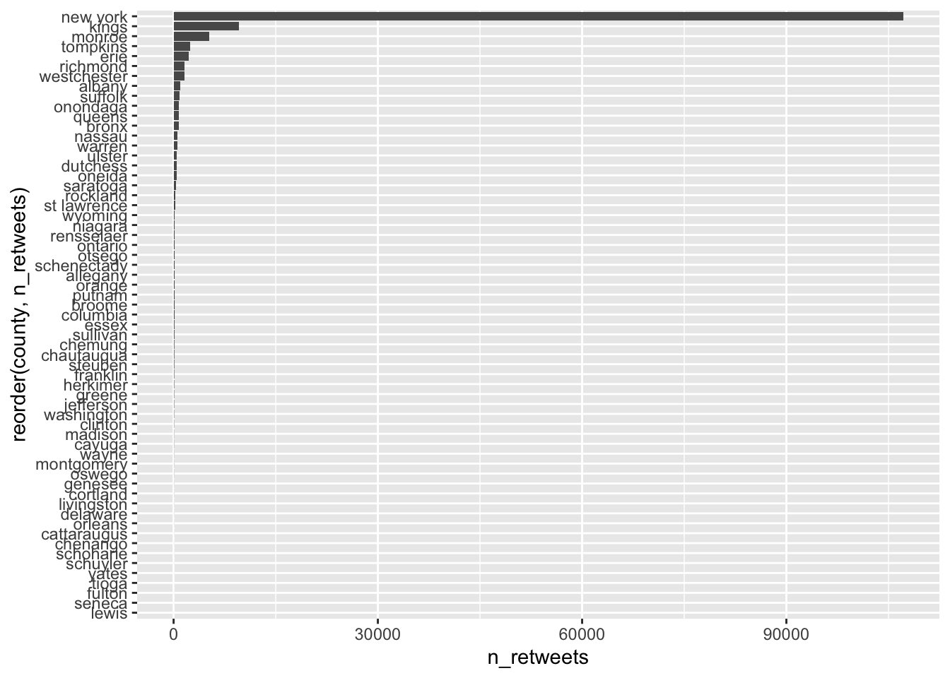
Describe the relationship between the number of retweets and
county using ggplot. Make a simple comment on your
plot.
Q1e <- NY_CC_tweets %>%
  group_by(county) %>%
summarize(n_retweets = n())ggplot(data = Q1e) +
geom_col(aes(x = n_retweets, y = county))
# Most retweets about #climatechange came from New York county.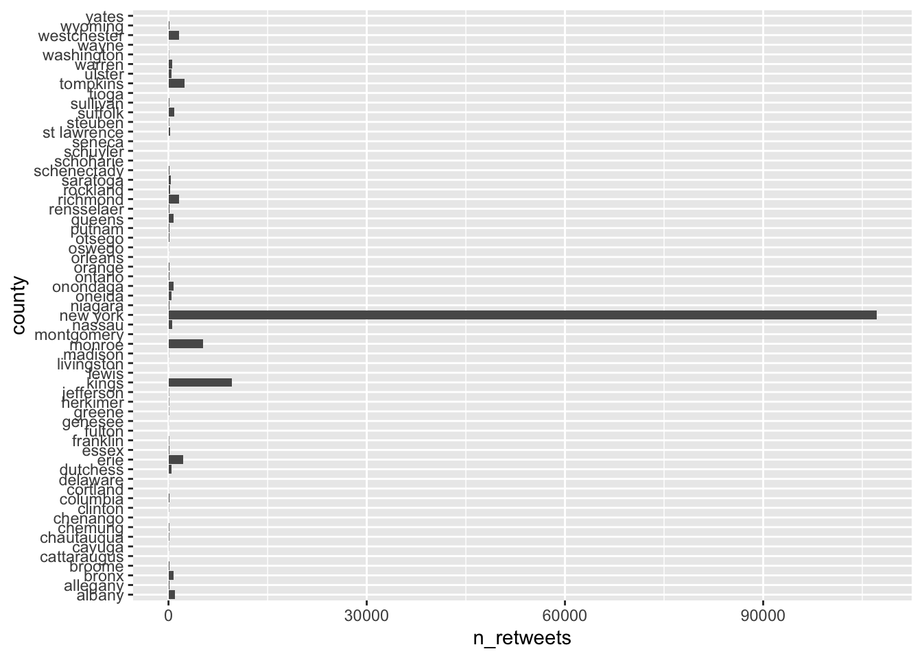
ggplot(data = Q1e) +
  geom_col(aes(x = n_retweets,
               y = reorder(county, n_retweets) ))
# reorder(CATEGORICAL_VAR, CONTINUOUS_VAR) reorders
# CATEGORICAL_VAR based on a values of CONTINUOUS_VAR