DANL 200: Introduction to Data Analytics
DANL 200 - Homework Assignment 4 - Example
Answers
Byeong-Hak Choe
2023-02-14
Loading R packages for Homework Assignment 4
library(tidyverse)
library(lubridate)
library(stargazer)
library(broom)
Question 1
Read the data file, bikeshare_cleaned.csv, as the
data.frame object with the name, bikeshare, using (1) the
read_csv() function and (2) its URL,
https://bcdanl.github.io/data/bikeshare_cleaned.csv.
url <- 'https://bcdanl.github.io/data/bikeshare_cleaned.csv'
bikeshare <- read_csv(url)
Use the data.frame bikeshare for the rest of questions
in Question 1.
- Description of variables in the data file, bikeshare_cleaned.csv
cnt: count of total rental bikesyear: yearmonth: monthdate: datehr: hourswkday: week dayholiday: holiday ifholiday== 1, non-holiday otherwiseseasons: seasonweather_cond: weather conditiontemp: temperature, measured in standard deviations from average.hum: humidity, measured in standard deviations from average.windspeed: wind speed, measured in standard deviations from average.
Q1a
Convert year, month, wkday,
hr, seasons, and weather_cond
into factor variables.
- Set
wkdayin order of ‘sunday’, ‘monday’, ‘tuesday’, etc. - Set
seasonsin order of ‘spring’, ‘summer’, ‘fall’, ‘winter’.
bikeshare <- bikeshare %>%
  mutate( year = factor(year),
          month = factor(month),
          hr = factor(hr),
          weather_cond = factor(weather_cond),
          wkday = factor(wkday,
                         levels = c("sunday", "monday", "tuesday", "wednesday",
                                    "thursday", "friday", "saturday") ),
          seasons = factor(seasons,
                           levels = c("spring", "summer", "fall", "winter") )
          )


levels(bikeshare$year)
## [1] "2011" "2012"levels(bikeshare$month)## [1] "01" "02" "03" "04" "05" "06" "07" "08" "09" "10" "11" "12"levels(bikeshare$hr)## [1] "0" "1" "2" "3" "4" "5" "6" "7" "8" "9" "10" "11" "12" "13" "14" "15" "16"
## [18] "17" "18" "19" "20" "21" "22" "23"levels(bikeshare$weather_cond)## [1] "Clear or Few Cloudy" "Light Snow or Light Rain" "Mist or Cloudy"levels(bikeshare$wkday)## [1] "sunday" "monday" "tuesday" "wednesday" "thursday" "friday" "saturday"levels(bikeshare$seasons)## [1] "spring" "summer" "fall" "winter"Q1b
Divide the bikeshare data.frame into training and
testing data.frames.
set.seed(20221121)
rn <- runif( nrow(bikeshare) )

# it is not necessary to do 50-50 split though
dtrain <- filter(bikeshare, rn >= .5)  # training data.frame
dtest <- filter(bikeshare, rn < .5)  # testing data.frame
Q1c
Train the linear regression model using the following
formula and the training data.frame.
Provide the summary of the regression result.
formula <-
  cnt ~ temp + hum + windspeed + weather_cond +
        hr + month + year
model <- lm(formula, data = dtrain)
summary(model)formula <-
cnt ~ temp + hum + windspeed + weather_cond +
hr + month + year
model <- lm(formula, dtrain)
stargazer(model, type = "html")| Dependent variable: | |
| cnt | |
| temp | 45.435*** |
| (2.497) | |
| hum | -16.002*** |
| (1.514) | |
| windspeed | -5.260*** |
| (1.192) | |
| weather_condLight Snow or Light Rain | -63.617*** |
| (4.554) | |
| weather_condMist or Cloudy | -9.905*** |
| (2.719) | |
| hr1 | -22.949*** |
| (7.539) | |
| hr2 | -30.672*** |
| (7.570) | |
| hr3 | -44.896*** |
| (7.600) | |
| hr4 | -46.209*** |
| (7.763) | |
| hr5 | -26.574*** |
| (7.516) | |
| hr6 | 33.192*** |
| (7.607) | |
| hr7 | 169.990*** |
| (7.633) | |
| hr8 | 313.340*** |
| (7.616) | |
| hr9 | 161.589*** |
| (7.563) | |
| hr10 | 102.764*** |
| (7.603) | |
| hr11 | 127.123*** |
| (7.733) | |
| hr12 | 165.599*** |
| (7.608) | |
| hr13 | 157.843*** |
| (7.727) | |
| hr14 | 148.061*** |
| (7.661) | |
| hr15 | 157.643*** |
| (7.769) | |
| hr16 | 214.809*** |
| (7.789) | |
| hr17 | 373.854*** |
| (7.621) | |
| hr18 | 345.954*** |
| (7.895) | |
| hr19 | 235.428*** |
| (7.602) | |
| hr20 | 153.243*** |
| (7.517) | |
| hr21 | 102.863*** |
| (7.632) | |
| hr22 | 65.298*** |
| (7.500) | |
| hr23 | 24.596*** |
| (7.526) | |
| month02 | 9.600* |
| (5.517) | |
| month03 | 32.520*** |
| (5.763) | |
| month04 | 50.391*** |
| (6.158) | |
| month05 | 61.240*** |
| (7.150) | |
| month06 | 45.513*** |
| (7.911) | |
| month07 | 18.049** |
| (8.588) | |
| month08 | 40.037*** |
| (8.183) | |
| month09 | 71.740*** |
| (7.357) | |
| month10 | 85.233*** |
| (6.371) | |
| month11 | 60.285*** |
| (5.686) | |
| month12 | 42.384*** |
| (5.542) | |
| year2012 | 84.498*** |
| (2.205) | |
| Constant | -8.347 |
| (7.693) | |
| Observations | 8,713 |
| R2 | 0.687 |
| Adjusted R2 | 0.685 |
| Residual Std. Error | 101.652 (df = 8672) |
| F Statistic | 475.432*** (df = 40; 8672) |
| Note: | p<0.1; p<0.05; p<0.01 |
Q1d
Which hr is most strongly associated with changes in
cnt? Interpret the beta estimate of that
hr.
sum_model <- tidy(model) %>%
  filter(str_detect(term, "hr")) %>%
  arrange(-estimate) %>%
  slice(1)
All else being equal, an
hour17relative to anhour0 is associated with an increase incntby \(373.85\).All else being equal, an
hour17relative to anhour0 is associated with an increase incntby \((373.85 - 2\times 7.62,\; 373.85 + 2\times 7.62)\).
Q1e
Make a prediction on the outcome variable using the testing data.frame and the regression result from Q1c.
dtest <- dtest %>%
  mutate( pred = predict(model,
                         newdata = dtest) )
Q1f
On average, are the predictions correct in the model in 3a? Are there systematic errors?
# actual vs. predicted outcome plot
ggplot( data = dtest,
        aes(x = pred, y = cnt) ) +
  geom_point( alpha = 0.2, color = "darkgray" ) +
  geom_smooth( color = "darkblue" ) +
  geom_abline( color = "red", linetype = 2 ) +  # y = x, perfect prediction line
  geom_vline(aes(xintercept = 0), lty = 'dotted') +
  geom_hline(aes(yintercept = 0), lty = 'dotted')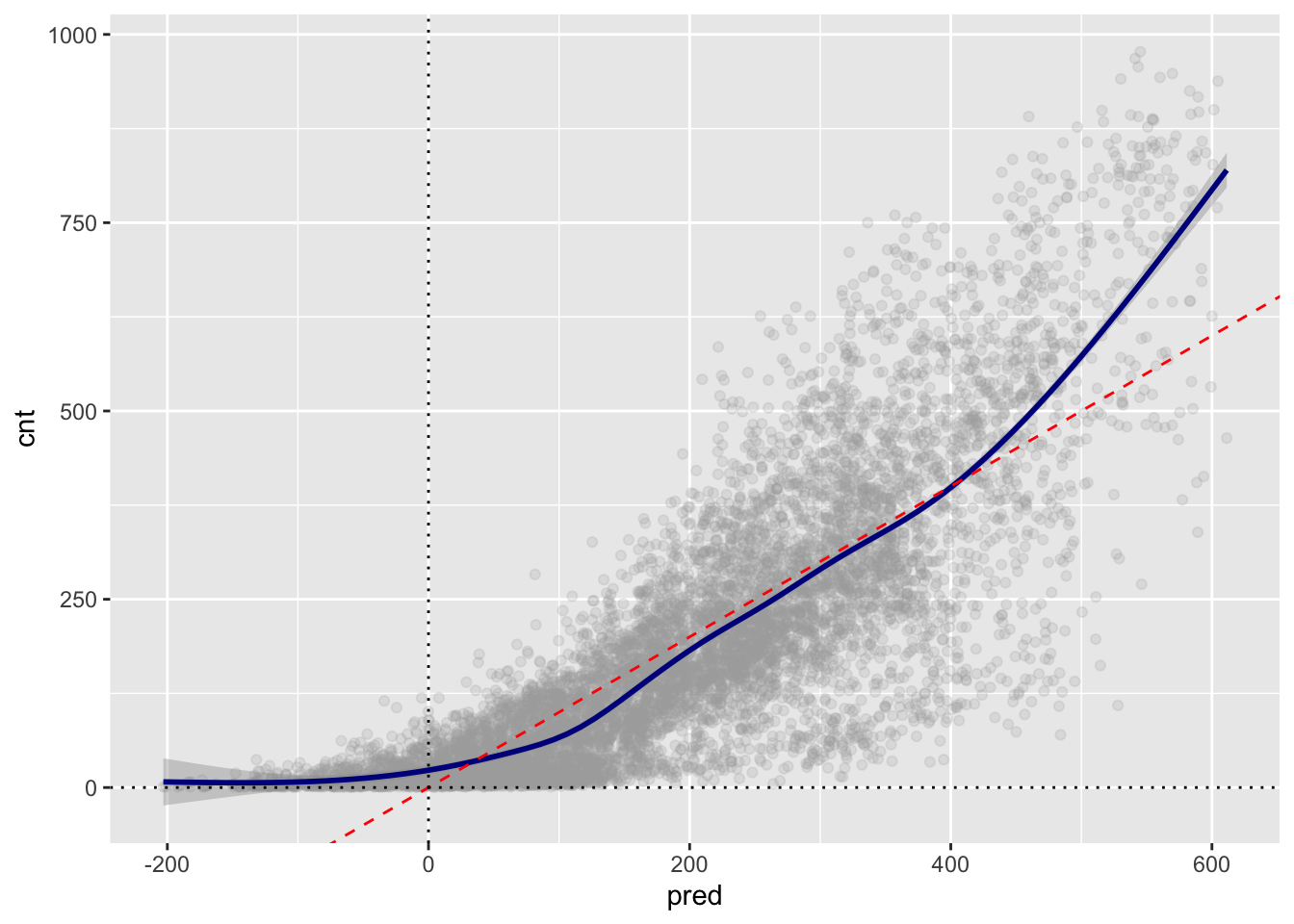
# resitual plot
ggplot(data = dtest,
       aes(x = pred, y = cnt - pred)) +
  geom_point(alpha = 0.2, color = "darkgray") +
  geom_smooth( color = "darkblue" ) +
  geom_hline( aes( yintercept = 0 ),  # perfect prediction
              color = "red", linetype = 2) +
  geom_vline(aes(xintercept = 0), lty = 'dotted')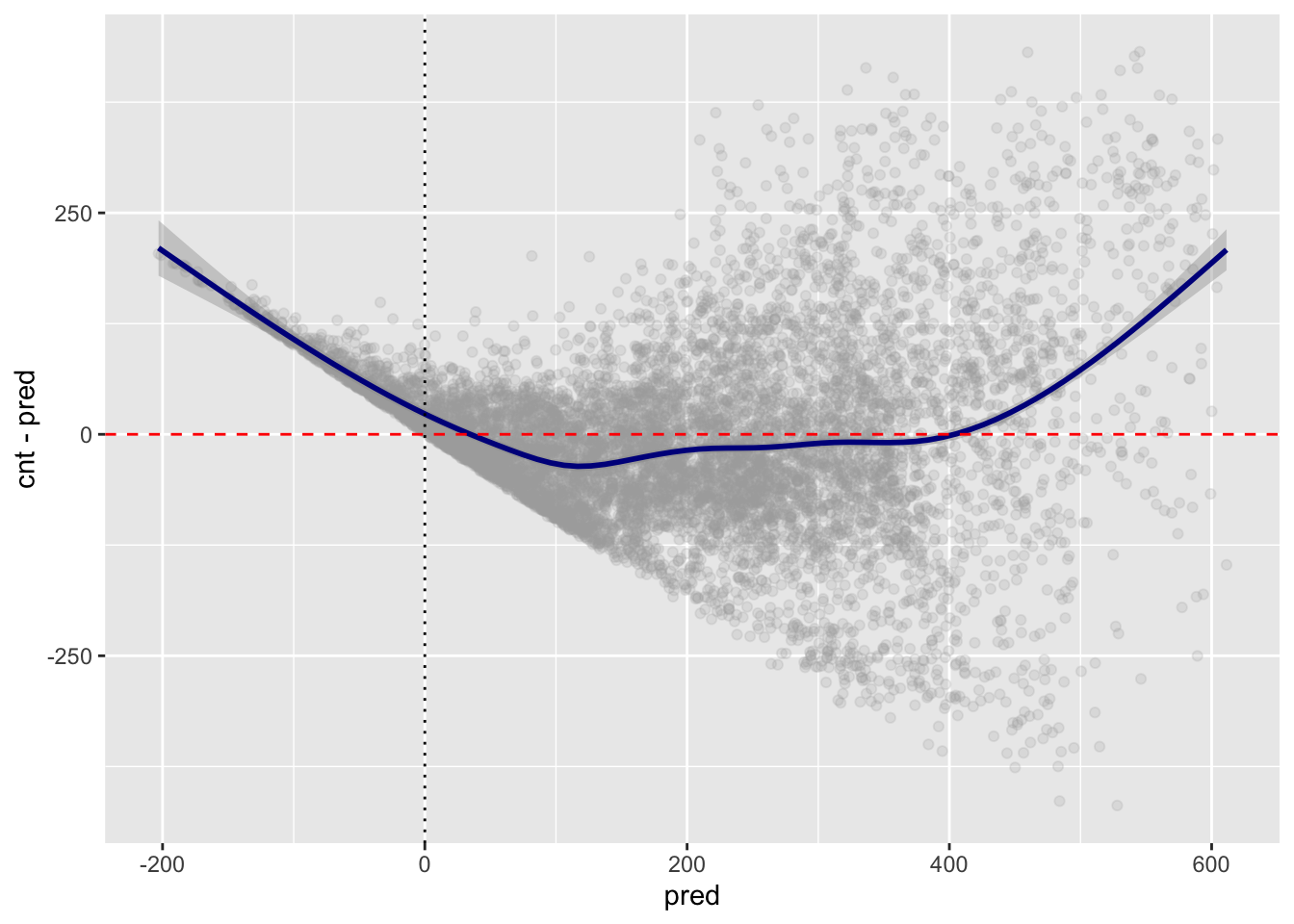
There is a systematic error in the sense that the variance of residual increases with the value of
pred.Additionally, some values of
predare less than zero, which may not make sense becausecnt\(\geq\) 0.