Loading R packages for Homework Assignment 2

library(tidyverse)

Question 1

Read the data file, NY_school_enrollment_socioecon.csv, as the data.frame object with the name, NY_school_enrollment_socioecon, using (1) the read_csv() function and (2) its URL, https://bcdanl.github.io/data/NY_school_enrollment_socioecon.csv.

url <- 'https://bcdanl.github.io/data/NY_school_enrollment_socioecon.csv'
NY_school_enrollment_socioecon <- read_csv(url)

For description of variables in NY_school_enrollment_socioecon, refer to the file, ny_school_enrollment_socioecon_description.zip, which is in the Files section in our Canvas web-page. (I recommend you to extract the zip file, and then read the file, ny_school_enrollment_socioecon_description.csv, using Excel or Numbers.)

Q1a

Look up the meaning of variables d01_018, d01_021, d01_024, and d01_027, from the file, ny_school_enrollment_socioecon_description.csv.

Find the top 5 counties in terms of the value of variable d01_018 for each year.
Find the top 5 counties in terms of the value of variable d01_021 for each year.
Find the top 5 counties in terms of the value of variable d01_024 for each year.
Find the top 5 counties in terms of the value of variable d01_027 for each year.
Make a comment on the result.

Q1a_25_34 <- NY_school_enrollment_socioecon %>% 
  select(year, county_name, d01_018) %>% 
  group_by(year) %>% 
  filter(min_rank(desc(d01_018)) <= 5) %>% 
  arrange(year, -d01_018)

Q1a_35_44 <- NY_school_enrollment_socioecon %>% 
  select(year, county_name, d01_021) %>% 
  group_by(year) %>% 
  filter(min_rank(desc(d01_021)) <= 5) %>% 
  arrange(year, -d01_021)

Q1a_45_64 <- NY_school_enrollment_socioecon %>% 
  select(year, county_name, d01_024) %>% 
  group_by(year) %>% 
  filter(min_rank(desc(d01_024)) <= 5) %>% 
  arrange(year, -d01_024)

Q1a_65_over <- NY_school_enrollment_socioecon %>% 
  select(year, county_name, d01_027) %>% 
  group_by(year) %>% 
  filter(min_rank(desc(d01_027)) <= 5) %>% 
  arrange(year, -d01_027)

# rank() and dense_rank() would also be okay.

# Here I do not provide any comments on the result.

Q1b

Look up the meaning of variables c02_010, c04_010, and c06_010 from the file, ny_school_enrollment_socioecon_description.csv.

Find the top 5 counties in terms of the value of variable c02_010 for each year.
Find the top 5 counties in terms of the value of variable c04_010 for each year.
Find the top 5 counties in terms of the value of variable c06_010 for each year.
Make a comment on the result.

Q1b_college <- NY_school_enrollment_socioecon %>% 
  select(year, county_name, c02_010) %>% 
  group_by(year) %>% 
  filter(min_rank(desc(c02_010)) <= 5) %>% 
  arrange(year, -c02_010)

Q1b_college_pub <- NY_school_enrollment_socioecon %>% 
  select(year, county_name, c04_010) %>% 
  group_by(year) %>% 
  filter(min_rank(desc(c04_010)) <= 5) %>% 
  arrange(year, -c04_010)

Q1b_college_prv <- NY_school_enrollment_socioecon %>% 
  select(year, county_name, c06_010) %>% 
  group_by(year) %>% 
  filter(min_rank(desc(c06_010)) <= 5) %>% 
  arrange(year, -c06_010)

# Here I do not provide any comments on the result.

Q1c

Look up the meaning of variable pincp from the file, ny_school_enrollment_socioecon_description.csv.

Provide both (1) one ggplot code with geom_line() and (2) a couple of sentences to describe the yearly trend of pincp for Livingston county and top 4 counties in terms of the mean value of pincp over the years, 2015-2020.

NY_school_enrollment_socioecon %>% 
  select(year, county_name, pincp) %>% 
  group_by(county_name) %>% 
  mutate( pincp_mean = mean(pincp) ) %>% 
  ungroup() %>% 
  filter( dense_rank(desc(pincp_mean)) <= 4 | 
            county_name == "Livingston" ) %>% 
  ggplot() +
  geom_line(aes(x = year, y = pincp, color = county_name)) +
  geom_point(aes(x = year, y = pincp, group = county_name))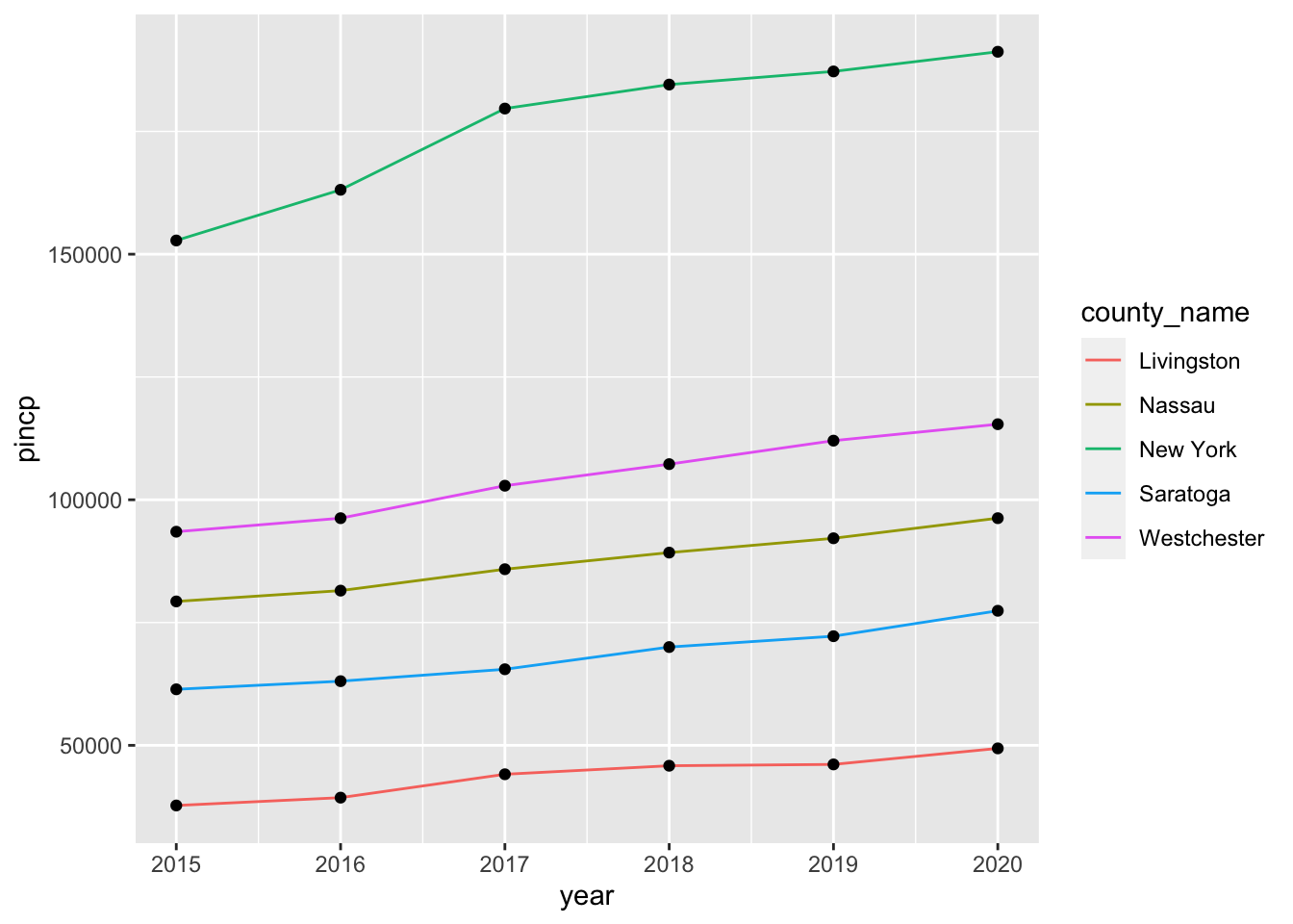

# Here I do not provide any comments on the result.

Q1d

Create the variable of the growth rate of pincp, where the growth rate of pincp is defined as:

\[ (\text{Growth rate of } \texttt{pincp} \text{ in year } \texttt{Y}) = \frac{( \texttt{pincp} \text{ in year } \texttt{Y} ) - ( \texttt{pincp} \text{ in year } \texttt{Y-1} )}{(\texttt{pincp} \text{ in year } \texttt{Y-1} )} \] Provide both (1) one ggplot code with geom_line() and (2) a couple of sentences to describe the yearly trend of the growth rate of pincp for Livingston county and top 5 counties in terms of the mean value of the growth rate of pincp over the years, 2016-2020.

NY_school_enrollment_socioecon %>% 
  select(year, county_name, pincp) %>% 
  group_by(county_name) %>% 
  mutate(g = 100 * (pincp - lag(pincp)) / lag(pincp),
         g_mean = mean(g, na.rm = T) ) %>% 
  ungroup() %>% 
  filter( (dense_rank(desc(g_mean)) <= 4 | 
            county_name == "Livingston") & !is.na(g) ) %>% 
  ggplot() +
  geom_line(aes(x = year, y = g, color = county_name)) +
  geom_point(aes(x = year, y = g, group = county_name))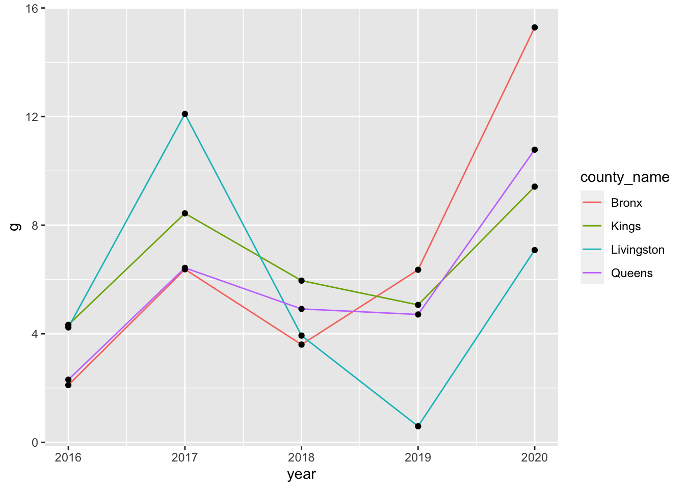

# Here I do not provide any comments on the result.

Q1e

Look up the meaning of variable poverty_hs and poverty_bachelor_or_higher from the file, ny_school_enrollment_socioecon_description.csv.

Summarize the mean value of poverty_hs and poverty_bachelor_or_higher from years 2015 to 2020 for each county.
Provide both (1) a ggplot code with geom_point() and (2) a couple of sentences to describe the mean value of poverty_hs.
Provide both (1) a ggplot code with geom_point() and (2) a couple of sentences to describe the mean value of poverty_bachelor_or_higher.

q1e <- NY_school_enrollment_socioecon %>% 
  group_by(county_name) %>% 
  summarise(poverty_hs = mean(poverty_hs),
            poverty_bachelor_or_higher = mean(poverty_bachelor_or_higher))

ggplot(q1e) +
  geom_point(aes(x = poverty_hs, 
                 y = county_name))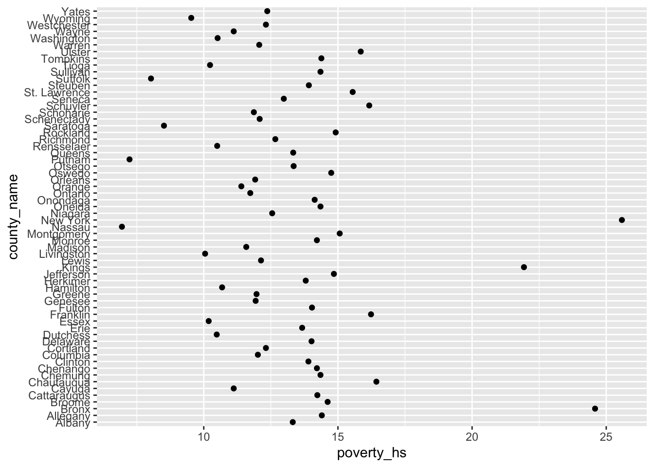

ggplot(q1e) +
  geom_point(aes(x = poverty_hs, 
                 y = reorder(county_name, poverty_hs)))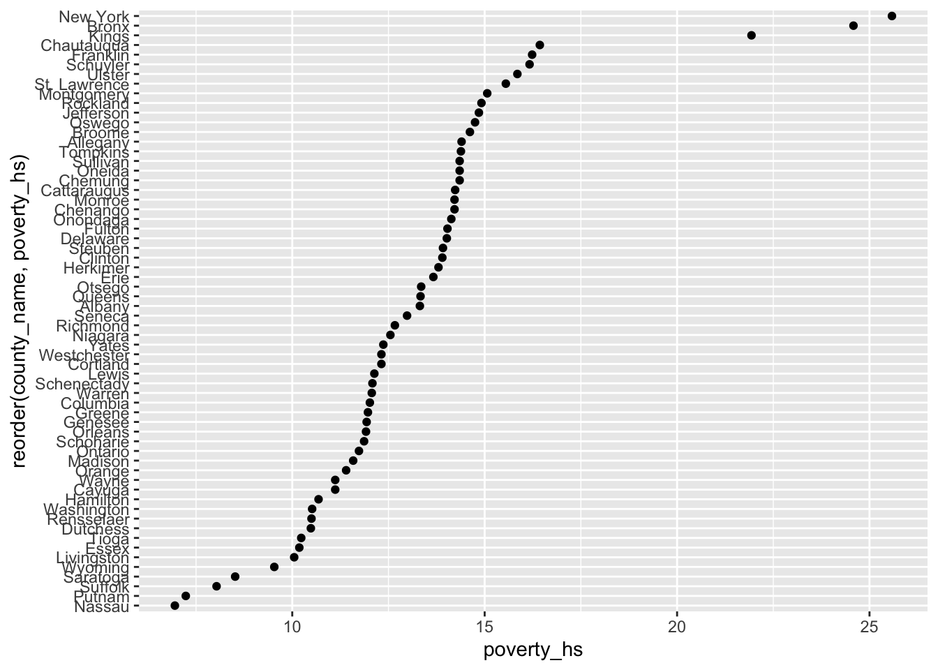

ggplot(q1e) +
  geom_point(aes(x = poverty_bachelor_or_higher, 
                 y = county_name))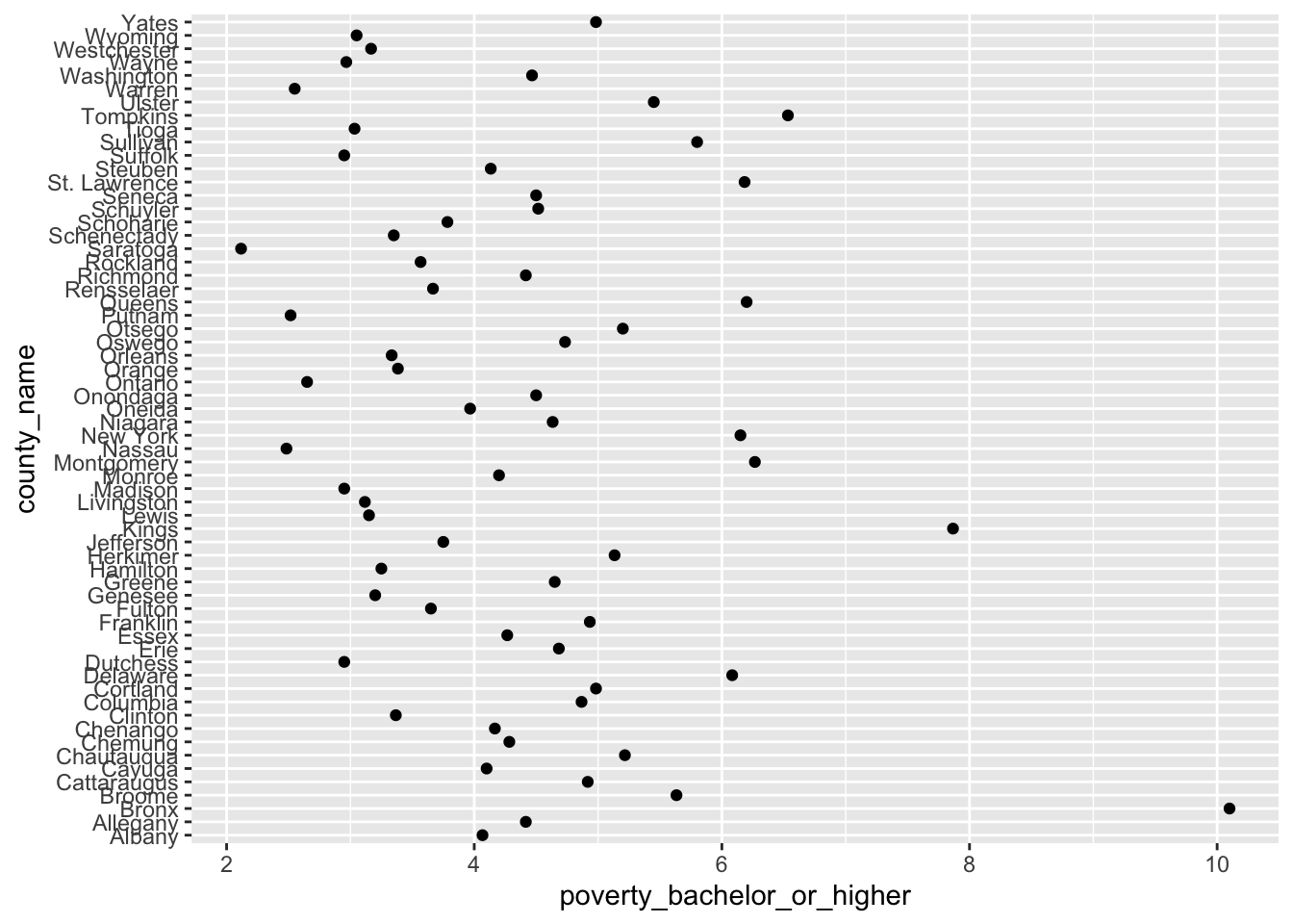

ggplot(q1e) +
  geom_point(aes(x = poverty_bachelor_or_higher, 
                 y = reorder(county_name, poverty_bachelor_or_higher)))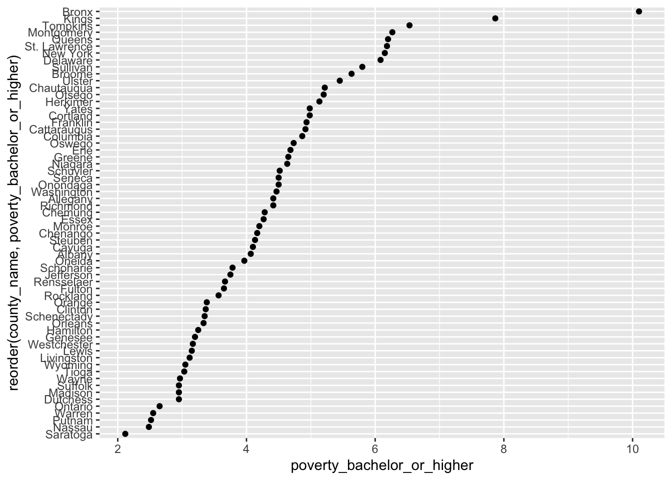

# Here I do not provide any comments on the result.

Question 2

Read the data file, beer_markets.csv, as the data.frame object with the name, beer_markets, using (1) the read_csv() function and (2) its URL, https://bcdanl.github.io/data/beer_markets.csv.

beer_markets <- read_csv(
  'https://bcdanl.github.io/data/beer_markets.csv'
)

Description of variables in the data file, `beer_markets.csv`

Each observation in beer_markets.csv is a household-level record for one transaction of beer.

hh: an identifier of the household;
X_purchase_desc: details on the purchased item;
quantity: the number of items purchased;
brand: Bud Light, Busch Light, Coors Light, Miller Lite, or Natural Light;
spent: total dollar value of purchase;
beer_floz: total volume of beer, in fluid ounces;
price_per_floz: price per fl.oz. (i.e., beer spent/beer floz);
container: the type of container;
promo: Whether the item was promoted (coupon or otherwise);
market: Scan-track market (or state if rural);
demographic data, including gender, marital status, household income, class of work, race, education, age, the size of household, and whether or not the household has a microwave or a dishwasher.

Q2a

Find the top 5 markets in terms of the total volume of beer.
Find the top 5 markets in terms of the total volume of BUD LIGHT.
Find the top 5 markets in terms of the total volume of BUSCH LIGHT.
Find the top 5 markets in terms of the total volume of COORS LIGHT.
Find the top 5 markets in terms of the total volume of MILLER LITE.
Find the top 5 markets in terms of the total volume of NATURAL LIGHT.

Q2a1 <- beer_markets %>% 
   group_by(market) %>% 
   summarize(beer_floz_tot = sum(beer_floz, na.rm = T)) %>% 
   arrange(-beer_floz_tot) %>% 
   slice(1:5)

Q2a_bud <- beer_markets %>% 
  filter(brand == "BUD LIGHT") %>% 
  group_by(market) %>% 
  summarize(beer_floz_tot = sum(beer_floz, na.rm = T)) %>% 
  arrange(-beer_floz_tot) %>% 
  slice(1:5)

Q2a_busch <- beer_markets %>% 
  filter(brand == "BUSCH LIGHT") %>% 
  group_by(market) %>% 
  summarize(beer_floz_tot = sum(beer_floz, na.rm = T)) %>% 
  arrange(-beer_floz_tot) %>% 
  slice(1:5)

Q2a_coors <- beer_markets %>% 
  filter(brand == "COORS LIGHT") %>% 
  group_by(market) %>% 
  summarize(beer_floz_tot = sum(beer_floz, na.rm = T)) %>% 
  arrange(-beer_floz_tot) %>% 
  slice(1:5)

Q2a_miller <- beer_markets %>% 
  filter(brand == "MILLER LITE") %>% 
  group_by(market) %>% 
  summarize(beer_floz_tot = sum(beer_floz, na.rm = T)) %>% 
  arrange(-beer_floz_tot) %>% 
  slice(1:5)

Q2a_natural <- beer_markets %>% 
  filter(brand == "NATURAL LIGHT") %>% 
  group_by(market) %>% 
  summarize(beer_floz_tot = sum(beer_floz, na.rm = T)) %>% 
  arrange(-beer_floz_tot) %>% 
  slice(1:5)

Q2b

For households that purchased BUD LIGHT, what fraction of households did purchase only BUD LIGHT?
For households that purchased BUSCH LIGHT, what fraction of households did purchase only BUSCH LIGHT?
For households that purchased COORS LIGHT, what fraction of households did purchase only COORS LIGHT?
For households that purchased MILLER LITE, what fraction of households did purchase only MILLER LITE?
For households that purchased NATURAL LIGHT, what fraction of households did purchase only NATURAL LIGHT?
Which beer brand does have the largest base of loyal consumers?

beer_markets <- beer_markets %>% 
  mutate(bud = ifelse(brand=="BUD LIGHT", 1, 0),
         busch = ifelse(brand=="BUSCH LIGHT", 1, 0),
         coors = ifelse(brand=="COORS LIGHT", 1, 0),
         miller = ifelse(brand=="MILLER LITE", 1, 0),
         natural = ifelse(brand=="NATURAL LIGHT", 1, 0) )

Q2b_bud <- beer_markets %>%
  select(hh, bud) %>%
  arrange(hh, -bud) %>%
  group_by(hh) %>%
  filter(sum(bud) > 0) %>% 
  mutate(frac_bud = sum(bud)/n(),
         loyal_bud = ifelse(frac_bud == 1, 1, 0)) %>%
  select(hh, frac_bud, loyal_bud) %>% 
  unique() %>% 
  ungroup() %>% 
  mutate(n_hh_bud = n()) %>%
  group_by(loyal_bud, n_hh_bud) %>% 
  summarise(n_obs = n()) %>% 
  ungroup() %>% 
  mutate(n_frac = n_obs/n_hh_bud )  # 0.6600816


Q2b_busch <- beer_markets %>%
  select(hh, busch) %>%
  arrange(hh, -busch) %>%
  group_by(hh) %>%
  filter(sum(busch) > 0) %>% 
  mutate(frac_busch = sum(busch)/n(),
         loyal_busch = ifelse(frac_busch == 1, 1, 0)) %>%
  select(hh, frac_busch, loyal_busch) %>% 
  unique() %>% 
  ungroup() %>% 
  mutate(n_hh_busch = n()) %>%
  group_by(loyal_busch, n_hh_busch) %>% 
  summarise(n_obs = n()) %>% 
  ungroup() %>% 
  mutate(n_frac = n_obs/n_hh_busch )  # 0.472973


Q2b_coors <- beer_markets %>%
  select(hh, coors) %>%
  arrange(hh, -coors) %>%
  group_by(hh) %>%
  filter(sum(coors) > 0) %>% 
  mutate(frac_coors = sum(coors)/n(),
         loyal_coors = ifelse(frac_coors == 1, 1, 0)) %>%
  select(hh, frac_coors, loyal_coors) %>% 
  unique() %>% 
  ungroup() %>% 
  mutate(n_hh_coors = n()) %>%
  group_by(loyal_coors, n_hh_coors) %>% 
  summarise(n_obs = n()) %>% 
  ungroup() %>% 
  mutate(n_frac = n_obs/n_hh_coors )  # 0.6390805


Q2b_miller <- beer_markets %>%
  select(hh, miller) %>%
  arrange(hh, -miller) %>%
  group_by(hh) %>%
  filter(sum(miller) > 0) %>% 
  mutate(frac_miller = sum(miller)/n(),
         loyal_miller = ifelse(frac_miller == 1, 1, 0)) %>%
  select(hh, frac_miller, loyal_miller) %>% 
  unique() %>% 
  ungroup() %>% 
  mutate(n_hh_miller = n()) %>%
  group_by(loyal_miller, n_hh_miller) %>% 
  summarise(n_obs = n()) %>% 
  ungroup() %>% 
  mutate(n_frac = n_obs/n_hh_miller )  # 0.6312989

Q2b_natural <- beer_markets %>%
  select(hh, natural) %>%
  arrange(hh, -natural) %>%
  group_by(hh) %>%
  filter(sum(natural) > 0) %>% 
  mutate(frac_natural = sum(natural)/n(),
         loyal_natural = ifelse(frac_natural == 1, 1, 0)) %>%
  select(hh, frac_natural, loyal_natural) %>% 
  unique() %>% 
  ungroup() %>% 
  mutate(n_hh_natural = n()) %>%
  group_by(loyal_natural, n_hh_natural) %>% 
  summarise(n_obs = n()) %>% 
  ungroup() %>% 
  mutate(n_frac = n_obs/n_hh_natural )  # 0.5096234

# Here I do not provide any comments on the result.

Q2c

Calculate the number of beer transactions for each household.
Calculate the fraction of each beer brand for each household.

Q2c <- beer_markets %>% 
  count(hh, brand) %>% 
  group_by(hh) %>% 
  mutate(n_tot = sum(n)) %>% 
  arrange(hh, brand) %>% 
  mutate( prop = n / n_tot )

DANL 200: Introduction to Data Analytics

DANL 200 - Homework Assignment 2 - Example Answers

Byeong-Hak Choe

2023-02-14

Loading R packages for Homework Assignment 2

Question 1

Q1a

Q1b

Q1c

Q1d

Q1e

Question 2

Description of variables in the data file, `beer_markets.csv`

Q2a

Q2b

Q2c

DANL 200: Introduction to Data Analytics

DANL 200 - Homework Assignment 2 - Example Answers

Byeong-Hak Choe

2023-02-14

Loading R packages for Homework Assignment 2

Question 1

Q1a

Q1b

Q1c

Q1d

Q1e

Question 2

Description of variables in the data file, beer_markets.csv

Q2a

Q2b

Q2c

Description of variables in the data file, `beer_markets.csv`