DANL 100: Programming for Data Analytics
DANL 100 - Homework Assignment 5 - Example
Answers
Byeong-Hak Choe
2023-02-14
- The following is the Python libraries we need for this homework.
import pandas as pd
import seaborn as sns
Question 1
Load the CSV file, beer_markets_cleaned.csv, from the
class website:
beer_markets = pd.read_csv('https://bcdanl.github.io/data/beer_markets_cleaned.csv')- Description of DataFrame
beer_markets- One single observation (row) corresponds to information regarding one household and its beer purchase.
- DataFrame
beer_marketsdoes not have any missing values.
- Variable (column) description
hh: an identifier of the household;purchase_desc: details on the purchased item;quantity: the number of items purchased;brand: Bud Light, Busch Light, Coors Light, Miller Lite, or Natural Light;spent: total dollar value of purchase;beer_floz: total volume of beer, in fluid ounces;price_per_floz: price per fl.oz. (i.e., beer spent/beer floz);container: the type of container;promo: Whether the item was promoted (coupon or otherwise);market: Scan-track market (or state if rural);- demographic data, including gender, marital status, household income, class of work, race, education, age, the size of household, and whether or not the household has a microwave or a dishwasher.
Q1a
- Sort the DataFrame
beer_marketsbyhhin ascending order.
Answer
beer_markets = beer_markets.sort_values('hh')Q1b
Count the number of households for each market.
Answer
# The below line counts the number of non-missing values
# for each variable for each group of "market" and "hh".
q1b = beer_markets.groupby(["market", "hh"]).count()

# In the resulting DataFrame q1b above,
# there is only one single observation for each group of
# "market" and "hh".
# So, the following line counts the number of households
# for each market.
q1b = q1b.groupby(["market"]).count()

q1b = q1b.loc[ :, ["brand"] ]
q1b.columns = ['n']   # rename `brand` with `n`

# For renaming, the following also works:
# q1b = q1b.rename({'brand':"n"}, axis = 'columns')
Q1c
Find the top 5 beer markets in terms of the number of households that purchased beer.
Answer
q1c = q1b.sort_values('n', ascending = False)| market | n |
|---|---|
| TAMPA | 280 |
| DETROIT | 214 |
| COLUMBUS | 184 |
| MIAMI | 178 |
| PHOENIX | 168 |
Q1d
Sum of beer_floz for each market.
Answer
q1d = beer_markets.groupby(["market"]).sum()
q1d = q1d.loc[ :, ["beer_floz"] ]

# the following gives the Series, instead of the DataFrame
# q1d = q1d['beer_floz']
Q1e
Find the top 5 beer markets in terms of the amount of total beer
consumption.
Answer
q1e = q1d.sort_values('beer_floz', ascending = False)| market | beer_floz |
|---|---|
| TAMPA | 462904 |
| PHOENIX | 388824 |
| DETROIT | 309588 |
| MIAMI | 271870 |
| COLUMBUS | 266896 |
Q1f
- Variable
price_per_flozis continuous. - Variable
brandis categorical.
Describe the distribution of price_per_floz for each
brand using seaborn.
Make a simple comment on comparison for the distribution of
price_per_floz across brands.
Answer
# distribution of price_per_floz for BUD LIGHT
sns.displot( x = 'price_per_floz', bins = 200,
             data = beer_markets[ beer_markets['brand'] == 'BUD LIGHT' ] )

# distribution of price_per_floz for COORS LIGHT
sns.displot( x = 'price_per_floz', bins = 200,
             data = beer_markets[ beer_markets['brand'] == 'COORS LIGHT' ] )

# distribution of price_per_floz for MILLER LITE
sns.displot( x = 'price_per_floz', bins = 200,
             data = beer_markets[ beer_markets['brand'] == 'MILLER LITE' ] )

# distribution of price_per_floz for BUSCH LIGHT
sns.displot( x = 'price_per_floz', bins = 200,
             data = beer_markets[ beer_markets['brand'] == 'BUSCH LIGHT' ] )

# distribution of price_per_floz for NATURAL LIGHT
sns.displot( x = 'price_per_floz', bins = 200,
             data = beer_markets[ beer_markets['brand'] == 'NATURAL LIGHT' ] )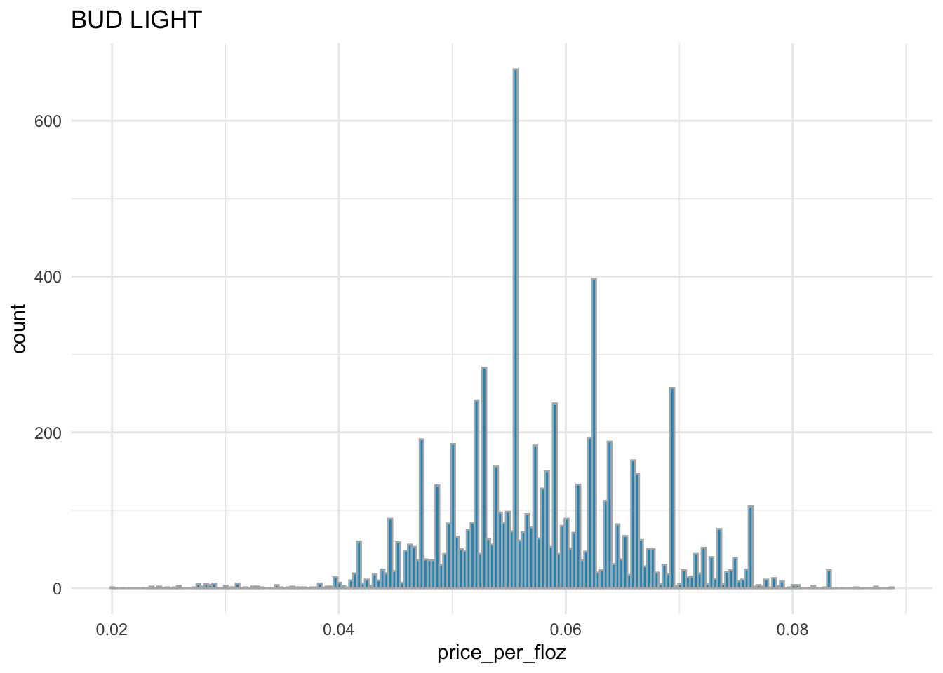
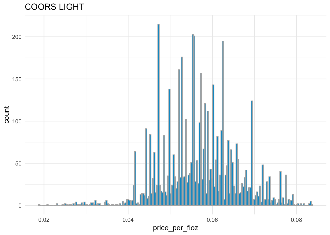
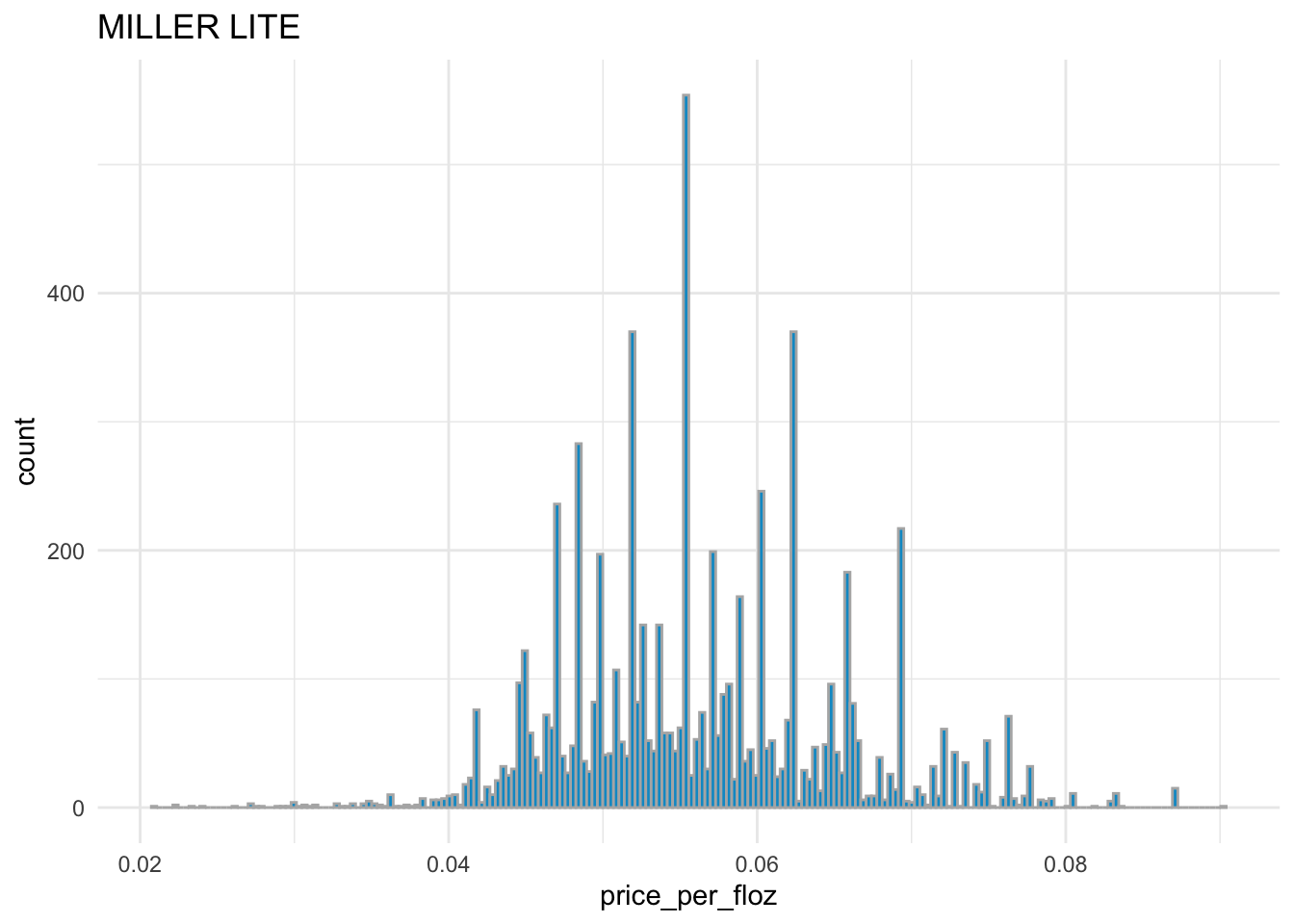
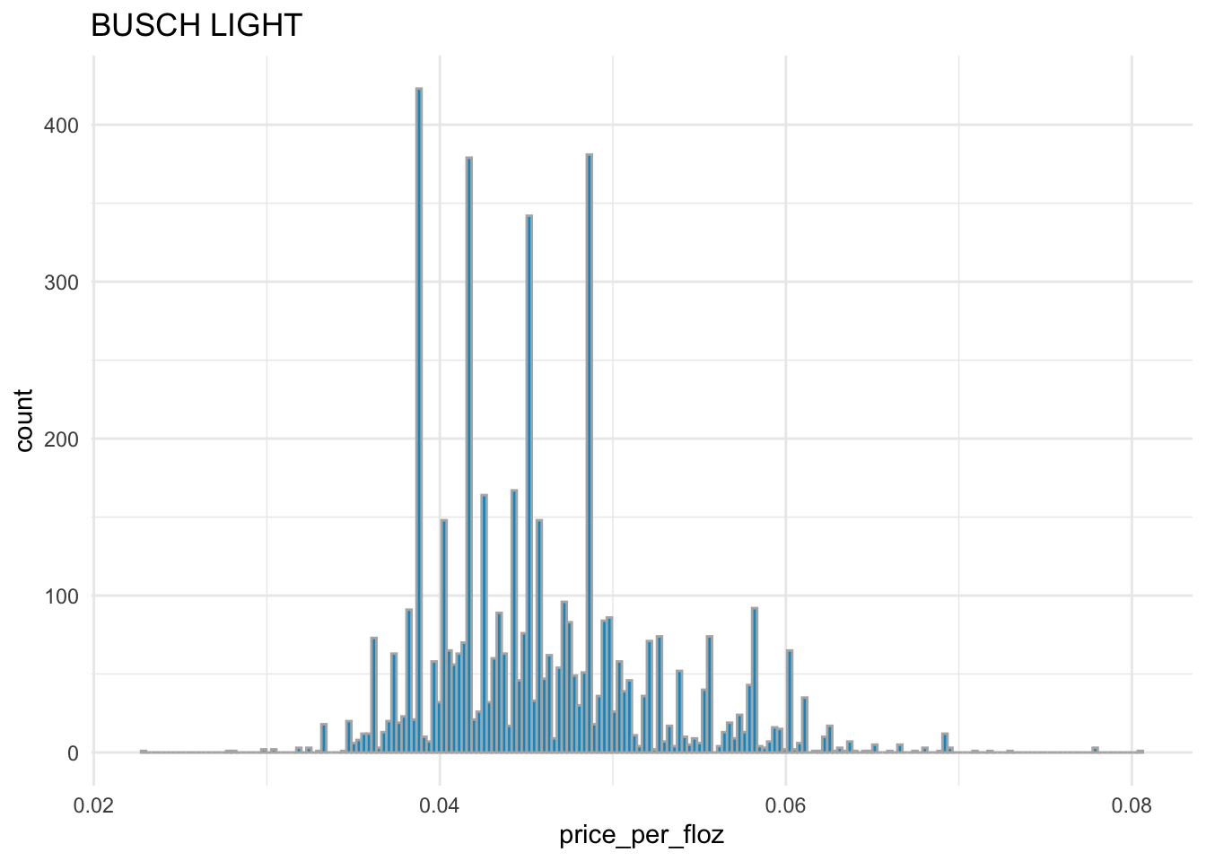
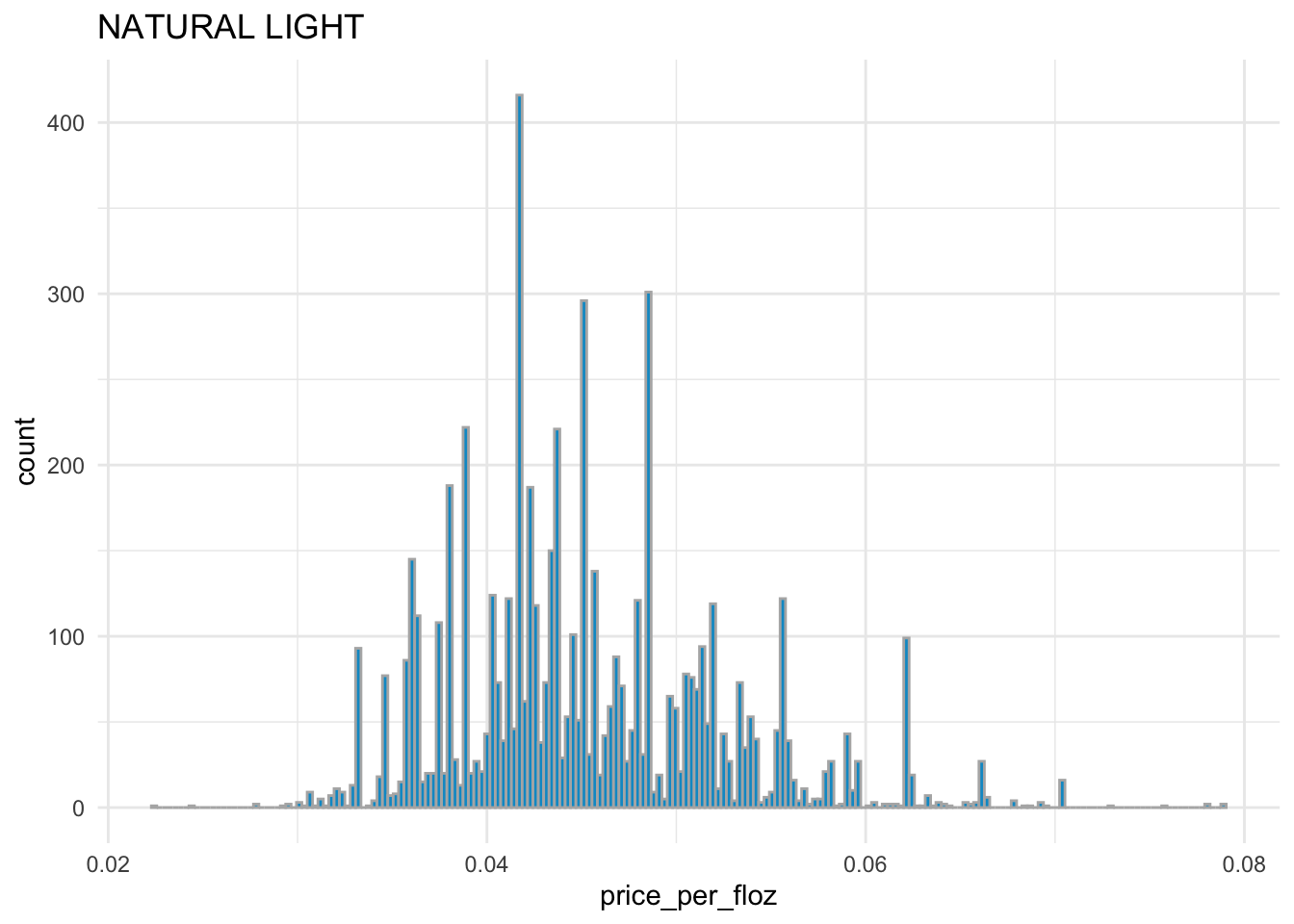
BUD LIGHT,COORS LIGHT, andMILLER LITEhave the similar distribution ofprice_per_flozwith each other.BUSCH LIGHTandNATURAL LIGHThave the similar distribution ofprice_per_flozwith each other.Overall,
BUD LIGHT,COORS LIGHT, andMILLER LITEare more expensive thanBUSCH LIGHTandNATURAL LIGHT.
Q1g
Both variables
price_per_flozandbeer_flozare continuous.Describe the relationship between
price_per_flozandbeer_flozby brand usingseaborn.Make a simple comment on the visualization result regarding how the relationship between
price_per_flozandbeer_flozvaries bybrand.
sns.lmplot(x = "beer_floz",
           y = "price_per_floz",
           scatter_kws = {'alpha' : 0.2},
           data = beer_markets[ beer_markets['brand'] == 'BUD LIGHT' ] )


sns.lmplot(x = "beer_floz",
           y = "price_per_floz",
           scatter_kws = {'alpha' : 0.2},
           data = beer_markets[ beer_markets['brand'] == 'COORS LIGHT' ] )


sns.lmplot(x = "beer_floz",
           y = "price_per_floz",
           scatter_kws = {'alpha' : 0.2},
           data = beer_markets[ beer_markets['brand'] == 'MILLER LITE' ] )


sns.lmplot(x = "beer_floz",
           y = "price_per_floz",
           scatter_kws = {'alpha' : 0.2},
           data = beer_markets[ beer_markets['brand'] == 'BUSCH LIGHT' ] )


sns.lmplot(x = "beer_floz",
           y = "price_per_floz",
           scatter_kws = {'alpha' : 0.2},
           data = beer_markets[ beer_markets['brand'] == 'NATURAL LIGHT' ] )


# all the plots in one plot:
sns.lmplot(x = "beer_floz",
           y = "price_per_floz",
           hue = "brand",
           scatter_kws = {'alpha' : 0.2},
           data = beer_markets)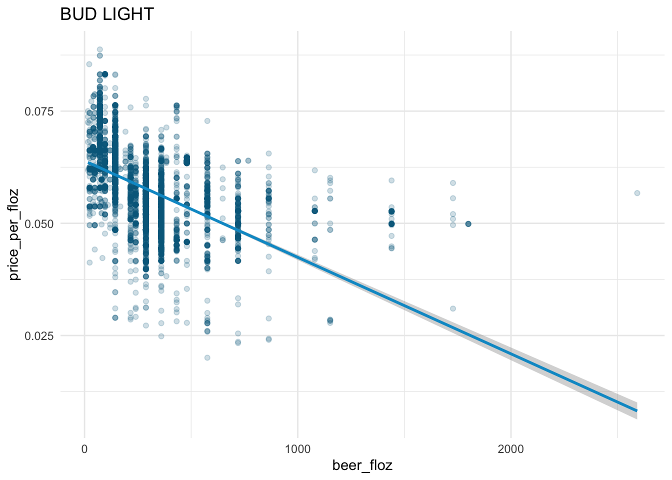
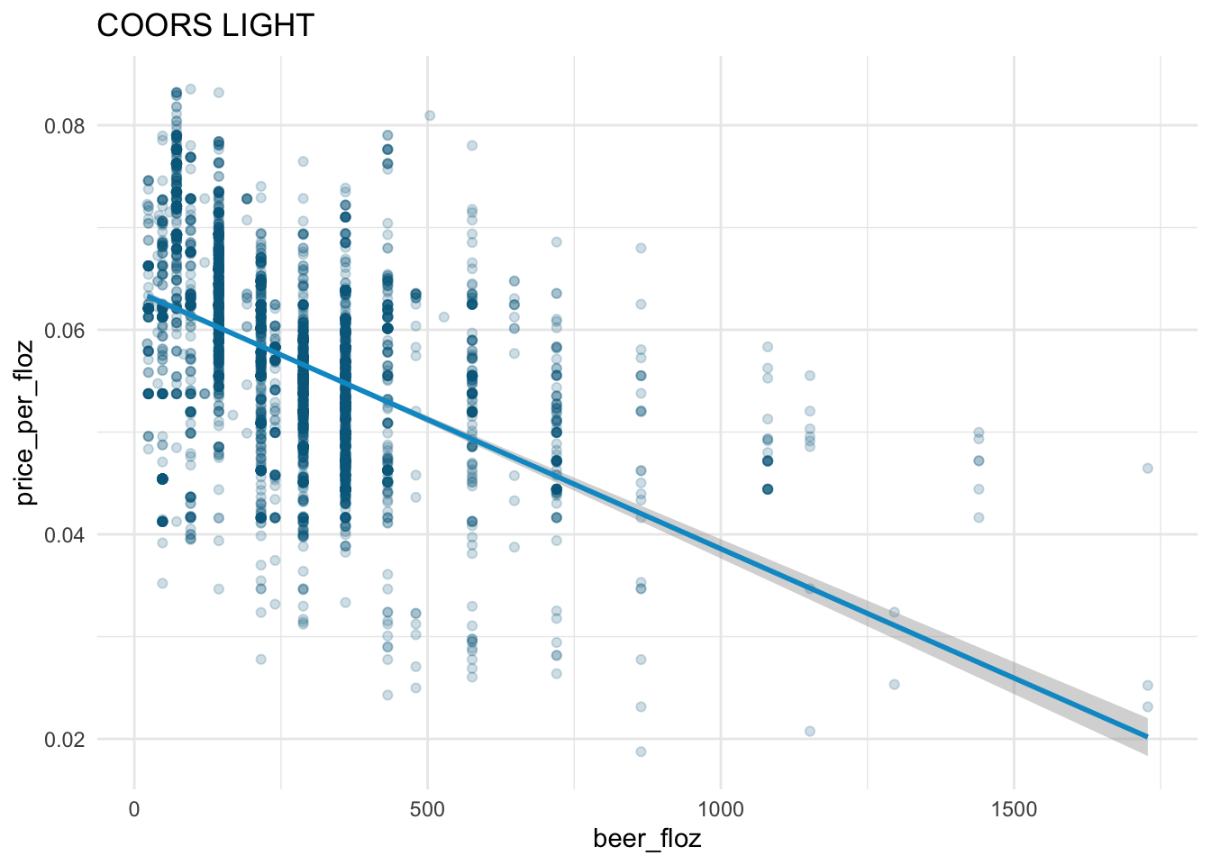
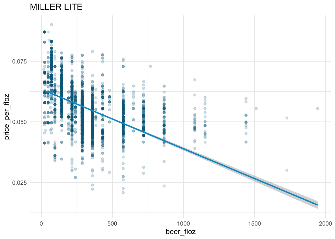
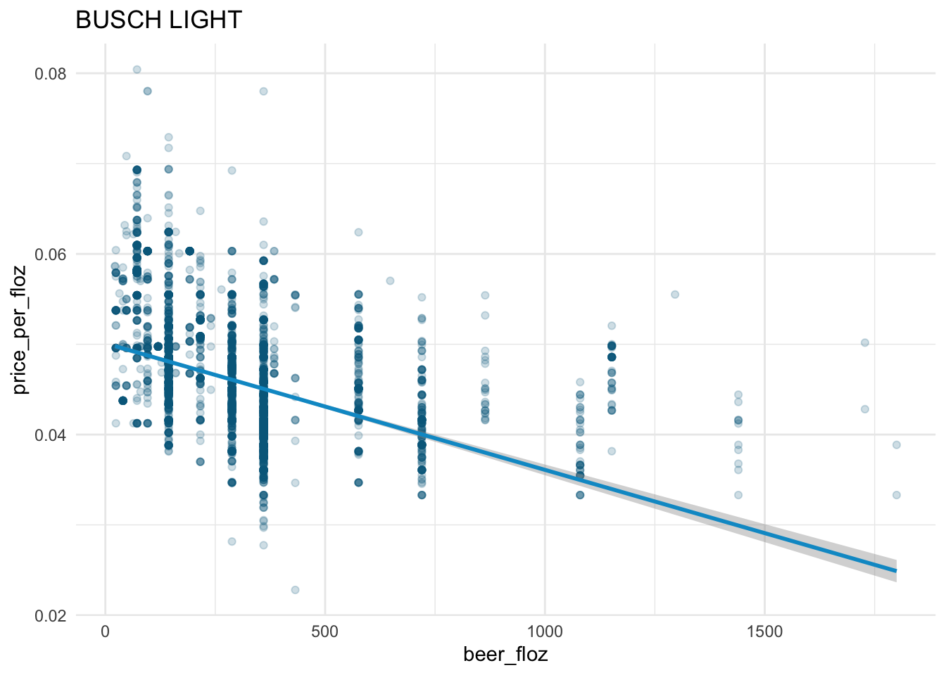
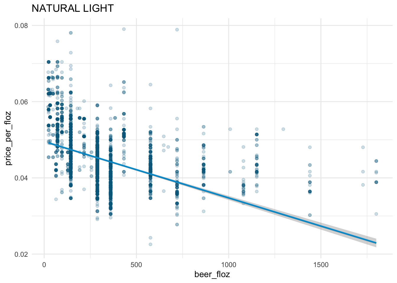
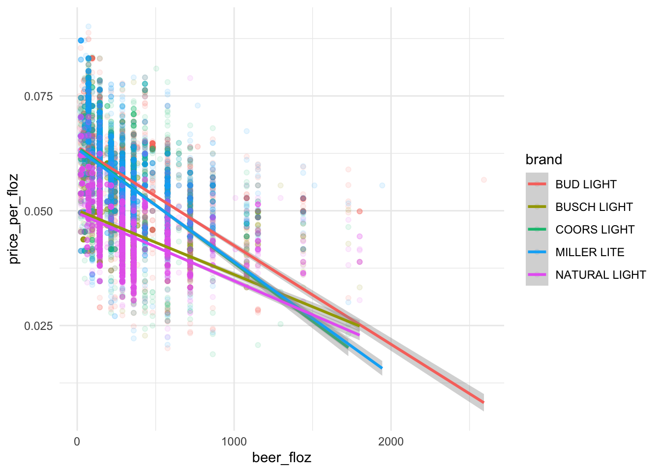
The law of demand holds in the beer market:
- From the fitted straight line, we see the downward-sloping demand curve for each beer brand.
The demand curves for
BUD LIGHT,COORS LIGHT, andMILLER LITEare steeper than those forBUSCH LIGHTandNATURAL LIGHT.According to the demand curves,
BUD LIGHT,COORS LIGHT, andMILLER LITEhave larger demands thanBUSCH LIGHTandNATURAL LIGHTgiven the same level ofprice_per_floz\(\geq\) 0.0375.