Lecture 25
DANL 200: Introduction to Data Analytics
Byeong-Hak Choe
December 1, 2022
Talk on Data Analytics Career

Lauren Kopac
Data Analyst, Human Capital Management (Compensation & Analytics)
Neuberger Berman
New York, NY June 2022 – Present
Talk on Data Analytics Career
Lauren Kopac
Assistant Director of Data, Law School in the Office of Academic Affairs
Institutional Research Analyst, School of Engineering in the Office of the Dean
Columbia University
New York, NY October 2018 – June 2022
Talk on Data Analytics Career
Lauren Kopac
MS Computer Science, Machine Learning
Columbia University
New York, NY Expected December 2023
BA Mathematics
SUNY Geneseo
Geneseo, NY August 2012 - December 2015
Announcement
Job Opportunities
- M&T guests, Leah Froebel and Emily Scheck
- Dec. 2nd (11:30 am - 12:30 pm) in South 340.
- All are welcome! They will be sharing their career stories along with an introduction to their F/T Management Development program (5 states) and prestigious internships in multiple functional areas (H/R, Marketing, Operations, etc...)
- McKinsey Consulting
- (F/T grad. Dec. '22 and May '23) 2-year paid rotational fellowship, NYC.
- If interested, send email to cannonm@geneseo.edu to meet with one of our McKinsey alumni for prep this week.
- Business Insights Fellow
- Blackstone
- (Econ. or Finance) Sophomore & Juniors,
- Apply to attend a Blackstone networking event in NYC, Jan. 13th 12:30 - 3:30 pm, application due 12/8.
- Blackstone Networking Event
Linear Regression using R
Linear Regression using R
More Explanatory Variables in the Model
In the 2016 US Census PUMS dataset, personal data recorded includes occupation, level of education, personal income, and many other demographic variables:
SCHL: level of education
Linear Regression using R
More Explanatory Variables in the Model
Suppose we also want to assess how personal income (
PINCP) varies with (1) age (AGEP), and (2) gender (SEX), and (3) a bachelor's degree (SCHL).- Conduct the exploratory data analysis.
- Based on the visualization, set a hypothesis regarding the relationship between having bachelor's degree and
PINCP. - Train the linear regression model.
- Interpret the beta coefficients from the linear regression result.
- Calculate the predicted
PINCPusing the testing data. - Draw the actual vs. predicted outcome plot and the residual plot.
Linear Regression in R
R commands to do EDA and linear regression analysis
library(tidyverse)psub <- readRDS( url('https://bcdanl.github.io/data/psub.RDS') )set.seed(54321)gp <- runif( nrow(psub) )# Set up factor variables if needed.dtrain <- filter(psub, gp >= .5)dtest <- filter(psub, gp < .5)library(skimr)sum_dtrain <- skim( select(dtrain, PINCP, AGEP, SEX, SCHL) )library(GGally)ggpairs( select(dtrain, PINCP, AGEP, SEX, SCHL) )# MORE VISUALIZATIONS ARE RECOMMENDEDmodel_1 <- lm( PINCP ~ AGEP + SEX, data = dtrain )model_2 <- lm( PINCP ~ AGEP + SEX + SCHL, data = dtrain )- Summary with base-R:
summary(model_1)summary(model_2)coef(model_1)coef(model_2)# Using the model.matrix() function on our linear model object, # we can get the data matrix that underlies our regression. df_model_1 <- as_tibble( model.matrix(model_1) )df_model_2 <- as_tibble( model.matrix(model_2) )- Summary with R packages:
# install.packages(c("stargazer", "broom"))library(stargazer)library(broom)stargazer(model_1, model_2, type = 'text') # from the stargazer packagesum_model_2 <- tidy(model_2) # from the broom package# Consider filter() to keep statistically significant beta estimatesggplot(sum_model_2) + geom_pointrange( aes(x = term, y = estimate, ymin = estimate - 2*std.error, ymax = estimate + 2*std.error ) ) + coord_flip()dtest <- dtest %>% mutate( pred_1 = predict(model_1, newdata = dtest), pred_2 = predict(model_2, newdata = dtest) )ggplot( data = dtest, aes(x = pred_2, y = PINCP) ) + geom_point( alpha = 0.2, color = "darkgray" ) + geom_smooth( color = "darkblue" ) + geom_abline( color = "red", linetype = 2 ) # y = x, perfect prediction lineggplot(data = dtest, aes(x = pred_2, y = PINCP - pred_2)) + geom_point(alpha = 0.2, color = "darkgray") + geom_smooth( color = "darkblue" ) + geom_hline( aes( yintercept = 0 ), # perfect prediction color = "red", linetype = 2)Linear Regression in R
The model equation
PINCP[i]=b0+b1*AGEP[i]+b2*SEX.Male[i]b3*SCHL.no high school diploma[i]+b4*SCHL.GED or alternative credential[i]+b5*SCHL.some college credit, no degree[i]+b6*SCHL.Associate's degree[i]+b7*SCHL.Bachelor's degree[i]+b8*SCHL.Master's degree[i]+b9*SCHL.Professional degree[i]+b10*SCHL.Doctorate degree[i]+e[i].
Linear Regression with Log-transformed Variables
Linear Regression with Log-transformtion
A Little Bit of Math for Logarithm
- The logarithm function, y=logb(x), looks like ....
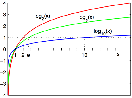
loge(x): the base e logarithm is called the natural log, where e=2.718⋯ is the mathematical constant, the Euler's number.
log(x) or ln(x): the natural log of x .
loge(7.389⋯): the natural log of 7.389⋯ is 2, because e2=7.389⋯.
Linear Regression with Log-transformtion
We should use a logarithmic scale when percent change, or change in orders of magnitude, is more important than changes in absolute units.
- For small changes in variable x from x0 to x1, the following equation holds:
Δlog(x)=log(x1)−log(x0)≈x1−x0x0=Δxx0.
- A change in income of $5,000 means something very different across people with different income levels.
- A percentage change in income, e.g., 5% of income, may mean somewhat more similar across people with different income levels.
- We can also consider using a log scale to reduce a variance of residuals when a variable is heavily skewed.
Linear Regression with Log-transformtion
- The log transformation makes the skewed distribution of income more normal.
ggplot(dtrain, aes( x = PINCP ) ) + geom_density() ggplot(dtrain, aes( x = log(PINCP) ) ) + geom_density()Linear Regression with Log-transformtion
A Few Algebras for Logarithm and Exponential Functions
- Rule 1:
y=log(x)⇔exp(y)=x.
- Rule 2:
log(x)−log(z)=log(xz).
- By the rules above,
log(x)−log(z)=b⇔xz=exp(b).
Linear Regression with Log-transformtion
- Let's consider the following linear regression model:
log(PINCP[i])=b0+b1*AGEP[i]+b2*SEX.Male[i]b3*SCHL.no high school diploma[i]+b4*SCHL.GED or alternative credential[i]+b5*SCHL.some college credit, no degree[i]+b6*SCHL.Associate's degree[i]+b7*SCHL.Bachelor's degree[i]+b8*SCHL.Master's degree[i]+b9*SCHL.Professional degree[i]+b10*SCHL.Doctorate degree[i]+e[i].
Linear Regression with Log-transformtion
Interpreting Beta Estimates
- If we apply the rule above for Bob and Ben's predicted incomes,
^log(PINCP[Ben])−^log(PINCP[Bob])=^b1 * (AGEP[Ben]−AGEP[Bob])=^b1 * (51 - 50)=^b1
So we can have the following: ^PINCP[Ben]^PINCP[Bob]=exp(^b1)⇔^PINCP[Ben]=^PINCP[Bob]∗exp(^b1)
Linear Regression with Log-transformtion
Interpreting Beta Estimates
- If we apply the rule above for Ben and Linda's predicted incomes,
^PINCP[Ben]^PINCP[Linda]=exp(^b2)⇔^PINCP[Ben]=^PINCP[Linda]∗exp(^b2)
Suppose exp(^b2)=1.18.
Then ^PINCP[Ben] is 1.18 times ^PINCP[Linda].
It means that being a male is associated with an increase in income by 18% relative to being a female.
Linear Regression with Log-transformtion
Interpreting Beta Estimates
All else being equal, an increase in
AGEPby one unit is associated with an increase inlog(PINCP)by ^b1.- All else being equal, an increase in
AGEPby one unit is associated with an increase inPINCPby (exp(^b1)−1)%.
- All else being equal, an increase in
All else being equal, being a male is associated with an increase in
log(PINCP)by ^b2 relative to being a female.- All else being equal, being a male is associated with an increase in
PINCPby (exp(^b2)−1)% relative to being a female.
- All else being equal, being a male is associated with an increase in
Linear Regression with Interaction Terms
Linear Regression with Interaction Terms
Motivation
Does the relationship between education and income vary by gender?
Suppose we are interested in knowing whether women are being compensated unequally despite having the same levels of education and preparation as men do.
How can linear regression address the question above?
Linear Regression with Interaction Terms
Model
- The linear regression with an interaction between explanatory variables X1 and X2 are:
Yi=b0+b1X1,i+b2X2,i+b3X1,i×X2,i+ei,
- where
- i: i-th observation in the training data.frame, i=1,2,3,⋯.
- Yi: i-th observation of outcome variable Y.
- Xp,i: i-th observation of the p-th explanatory variable Xp.
- ei: i-th observation of statistical error variable.
Linear Regression with Interaction Terms
Model
- The linear regression with an interaction between explanatory variables X1 and X2 are:
Yi=b0+b1X1,i+b2X2,i+b3X1,i×X2,i+ei
- The relationship between X1 and Y is now described by not only b1 but also b3X2:
ΔYΔX1=b1+b3X2
Linear Regression with Interaction Terms
Motivation
- Is education related with income?
model <- lm( log(PINCP) ~ AGEP + SCHL + SEX, data = dtrain )- Does the relationship between education and income vary by gender?
model_int <- lm( log(PINCP) ~ AGEP + SCHL + SEX + SCHL * SEX, data = dtrain )# Equivalently,model_int <- lm( log(PINCP) ~ AGEP + SCHL * SEX, # Use this one data = dtrain )Log-Log Linear Regression
Log-Log Linear Regression
Estimating Price Elasticity
- To estimate the price elasticity of orange juice (OJ), we will use sales data for OJ from Dominick’s grocery stores in the 1990s.
- Weekly
priceandsales(in number of cartons "sold") for three OJ brands---Tropicana, Minute Maid, Dominick's - An indicator,
feat, showing whether eachbrandwas advertised (in store or flyer) that week.
- Weekly
| Variable | Description |
|---|---|
sales |
Quantity of OJ cartons sold |
price |
Price of OJ |
brand |
Brand of OJ |
feat |
Advertisement status |
Log-Log Linear Regression
Estimating Price Elasticity
- Let's prepare the OJ data:
oj <- read_csv('https://bcdanl.github.io/data/dominick_oj.csv')# Split 70-30 into training and testing data.framesset.seed(14454)gp <- runif( nrow(oj) )dtrain <- filter(oj, [?])dtest <- filter(oj, [?])Log-Log Linear Regression
Estimating Price Elasticity
- The following model estimates the price elasticity of demand for a carton of OJ:
log(salesi)=b0+btrbrandtr,i+bmmbrandmm,i+b1log(pricei)+ei
- where
brandtr,i ={1 if an orange juice i is Tropicana;0otherwise.
brandmm,i ={1 if an orange juice i is Minute Maid;0otherwise.
Log-Log Linear Regression
Estimating Price Elasticity
- The following model estimates the price elasticity of demand for a carton of OJ:
log(salesi)=b0+btrbrandtr,i+bmmbrandmm,i+b1log(pricei)+ei
When brandtr,i=0 and brandmm,i=0, the beta coefficient for the intercept b0 gives the value of Dominick's log sales at a log price of zero.
The beta coefficient b1 is the price elasticity of demand.
- It measures how sensitive the quantity demanded is to its price.
Log-Log Linear Regression
Estimating Price Elasticity
- For small changes in variable x from x0 to x1, the following equation holds:
Δlog(x)=log(x1)−log(x0)≈x1−x0x0=Δxx0.
- The coefficient on log(pricei), b1, is therefore
b1=Δlog(salesi)Δlog(pricei)=ΔsalesisalesiΔpriceipricei,
the percentage change in sales when price increases by 1%.
Log-Log Linear Regression
Estimating Price Elasticity
- Let's train the model:
log(salesi)=b0+btrbrandtr,i+bmmbrandmm,i+b1log(pricei)+ei
reg_1 <- lm([?], data = dtrain)