Lecture 2
DANL 200: Introduction to Data Analytics
Byeong-Hak Choe
Septermber 1, 2022
Announcement
Changes in Office Hours
- Office: South Hall 117B.
- Office Hours:
- Mondays 3:30 PM-5:30 PM
- Wednesdays 1:30 PM-3:30 PM.
Installing the Tools
Installing the Tools
R programming
The R language is available as a free download from the R Project website at:
- Windows: https://cran.r-project.org/bin/windows/base/
- Mac: https://cran.r-project.org/bin/macosx/
- Download the file of R that corresponds to your Mac OS (Big Sur, Apple silicon arm64, High Sierra, El Capitan, Mavericks, etc.)
Installing the Tools
RStudio
RStudio offers a graphical interface to assist in creating R code:
- The RStudio Desktop is available as a free download from the following webpage:
- https://www.rstudio.com/products/rstudio/download/#download
Installing the Tools
RStudio Environment
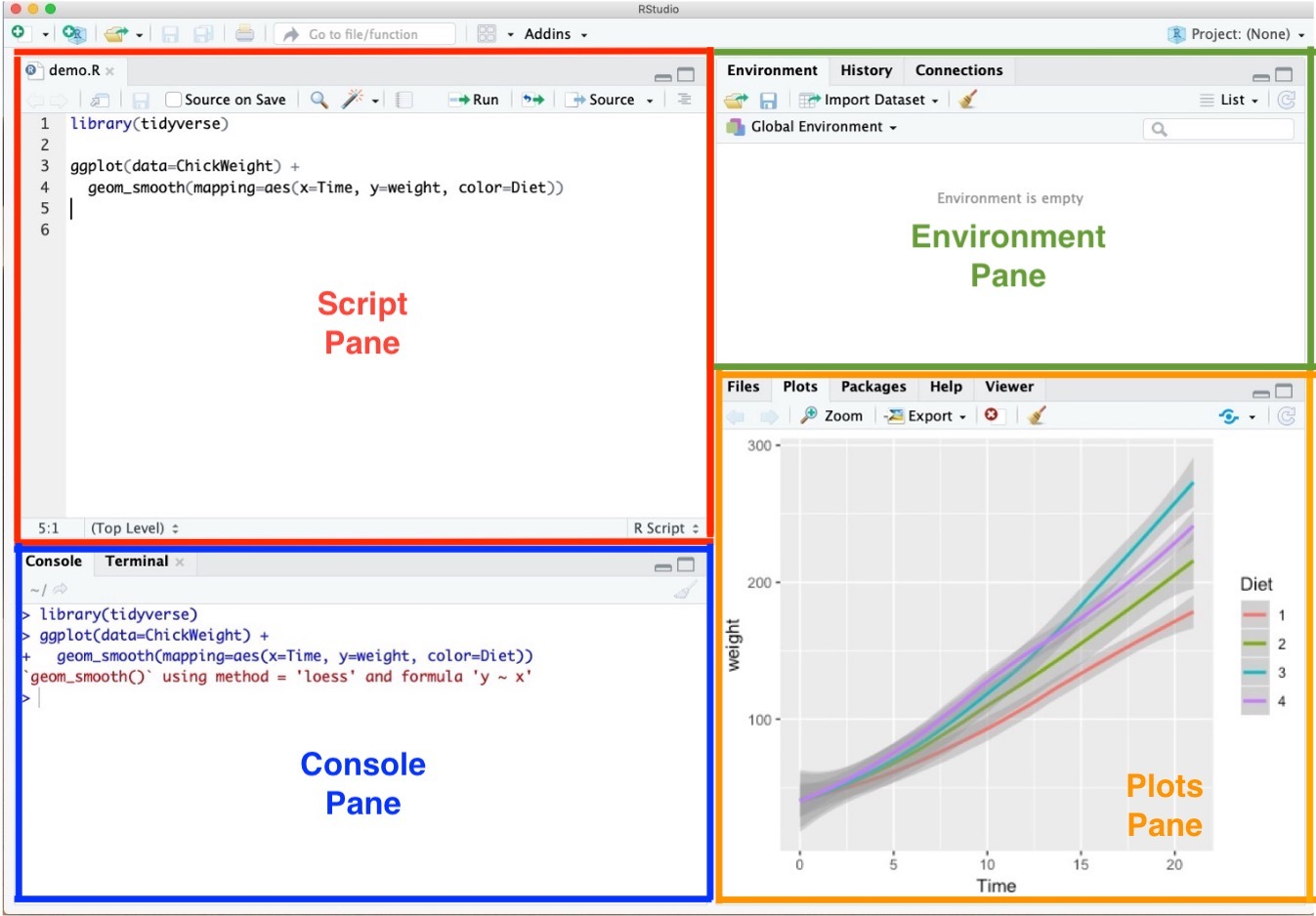
- Script Pane is where you write R commands in a script file that you can save.
- An R script is simply a text file containing R commands.
- RStudio will color-code different elements of your code to make it easier to read.
Installing the Tools
RStudio Environment
- Console Pane allows you to interact directly with the R interpreter and type commands where R will immediately execute them.
Installing the Tools
RStudio Environment
- Environment Pane is where you can see the values of variables, data frames, and other objects that are currently stored in memory.
Installing the Tools
RStudio Environment
- Plots Pane contains any graphics that you generate from your R code.
Installing the Tools
RStudio Environment
# Answer "no" to:# Do you want to install from sources the packages which need compilation?update.packages(ask = FALSE, checkBuilt = TRUE)pkgs <- c("tidyverse", "nycflights13", "gapminder", "skimr")install.packages(pkgs, dependencies = c("Depends", "Imports", "LinkingTo"))Management of Files, Directories, and Scripts
Management of Files, Directories, and Scripts
Materials for the book, Practical Data Science with R
- Click the green "Code" button and download the ZIP file from the following GitHub page: https://github.com/WinVector/PDSwR2.
- Step 1. Go to your Download folder (or the folder where the downloaded file is saved) using the File Explorer.
- Step 2. Click the ZIP file one time.
- Step 3. Cut the file by using the shortcut (Ctrl+X).
- Step 4. Go to your working folder for the course using the File Explorer.
- Step 5. Paste the file to your working folder by using Ctrl+V.
- Step 6. Right-click the ZIP file and click "Extract ..."
- Step 1. Go to your Download folder (or the folder where the downloaded file is saved) using the Finder.
- Step 2. Click the ZIP file (or the folder if the ZIP file is extracted) one time.
- Step 3. Copy the file (or the folder) by using the shortcut (command+C).
- Step 4. Go to your working folder for the course using the Finder.
- Step 5. Paste the file to your working folder by using command+option+V.
- Step 6. Right-click the ZIP file and click "Extract ..."
Management of Files and Directories
Finding the path name of the file
- Step 1. Go to your folder using the File Explorer.
- Step 2. Right-click the file.
- Step 3. Click "Copy as path".
- Step 4. Paste the path name of the file to the R script (Ctrl+V).
- Step 5.
- Option 1. Replace backslash(
\) with double-backslash(\\) in the path name. - Option 2. Add
rat the beginning of the path name: - 'r PATH_FOR_YOUR_FILE'.
- Option 1. Replace backslash(
- Step 1. Go to your folder using the File Explorer.
- Step 2. Keep pressing the "Shift" key
- Step 3. Right-click the file.
- Step 4. Click "Copy as path".
- Step 5. Paste the path name of the file to the R script (Ctrl+V).
- Step 6.
- Option 1. Replace backslash(
\) with double-backslash(\\) in the path name. - Option 2. Add
rat the beginning of the path name: - 'r PATH_FOR_YOUR_FILE'.
- Option 1. Replace backslash(
- Step 1. Go to your folder using the Finder.
- Step 2. Right-click the file in the folder
- Step 3. Keep pressing "option"
- Step 4. Click "Copy 'PATH_FOR_YOUR_FILE' as Pathname" from the menu.
- Step 5. Paste it to the R script (command+V).
Management of Files, Directories, and Scripts
Code and comment style
The two main principles for coding and managing data are:
- Make things easier for your future self.
- Don't trust your future self.
The
#mark is R's comment character.#indicates that the rest of the line is to be ignored.- Write comments before the line that you want the comment to apply to.
Consider using block commenting for separating code sections.
####defines a coding block.
Break down long lines and long algebraic expressions.
Starting with R
Starting with R
RStudio Options Setting

- This option menu is found by menus as follows:
- Mac: RStudio > Preferences
- Windows: Tools > Global Options
Starting with R
- Let's try a few commands to help you become familiar with R and its basic data types.
11/2'Joe'"Joe""Joe"=='Joe'c()is.null(c())is.null(5)- In R, vectors are arrays of same-typed values.
- They can be built with the
c()notation.
- They can be built with the
c(1)c(1, 2)c("Apple", 'Orange')length(c(1, 2))vec <- c(1, 2)vecStarting with R
Code and comment style
- R has many assignment operators (e.g.,
<-,=,->). - The preferred one is
<-.
x <- 2x < - 3print(x)x <- 5x = 55 -> xStarting with R
Shortcuts
Mac
- command + return runs a current line (where the blinking cursor is) or selected lines.
- command + shift + C is the shortcut for #.
- option + - is the shortcut for
<-.
Windows
- Ctrl + Enter runs a current line (where the blinking cursor is) or selected lines.
- Ctrl + Shift + C is the shortcut for #.
- Alt + - is the shortcut for
<-.
Starting with R
R data types
- Primary data types in R are as follows:
- Logical: A simple binary variable that may have only two values---TRUE or FALSE.
- Numeric: Decimal numbers
- Integer: Integers
- Character: Text strings
- Factor: Categorical values. Each possible value of a factor is known as a level.
- Ordered Factor: A special factor data type where the order of the levels is significant. E.g., Low, Medium, and High
Starting with R
R data types
- Test the data types.x <- TRUEy <- 1z <- 'Data Analytics'productCategory <- c('fruit', 'vegetable', 'dry goods', 'fruit','vegetable', 'dry goods')productCategoryFactor <- factor(productCategory)
- The
class()function returns the data type of an object.- What are classes for
x,y,z,productCategory, andproductCategoryFactor?
- What are classes for
Starting with R
R data types
- Most R data types are mutable, in that we're allowed to change them.
a <- c(1, 2)b <- aprint(b)# Alters aa[[1]] <- 5print(a)print(b)Starting with R
Lists
- Lists, unlike vectors, can store more than one type of object.
- The ways to access items in lists are the
$operator and the[[]]operator.
- The ways to access items in lists are the
x <- list('a' = 6, b = 'fred')names(x)x$ax$bx[['a']]x[c('a', 'a', 'b', 'b')]Starting with R
R data types
- Here are examples of a vector and a list.
example_vector <- c(10, 20, 30)example_list <- list(a = 10, b = 20, c = 30)example_vector[1]example_list[1]example_vector[[2]]example_list[[2]]example_vector[c(FALSE, TRUE, TRUE)]example_list[c(FALSE, TRUE, TRUE)]example_list$bexample_list[["b"]]Starting with R
Errors
Errors are just R's way of saying it safely refused to complete an ill-formed operation
Fear of errors should not limit experiments.
x <- 1:5print(x)x <- meanMISSPELLED(x) print(x) x <- mean(x) print(x)Starting with R
Data Frames
- R’s central data structure is the data frame.
- A data frame is organized into rows and columns.
- Data frames are essentially lists of columns.
- Data frames can have columns of different types.
d <- data.frame(x=c(1,2), y=c('a','b'))d[['x']]d$xd[[1]]dd[1,]d[,1]d[1,1]d[1, 'x']Starting with R
Data Frames
- The R data.frame class is designed to store data in a very good "ready for analysis" format.
d <- data.frame(col1 = c(1, 2, 3), col2 = c(-1, 0, 1))print(d)d$col3 <- d$col1 + d$col2print(d)Starting with R
NULL and NA values
NULLis just an alias forc(), the empty vector.NAindicates missing or unavailable data.
c(c(), 1, NULL)c("a", NA, "c")Starting with R
NULL and NA values
NULLis just an alias forc(), the empty vector.NAindicates missing or unavailable data.
c(c(), 1, NULL)c("a", NA, "c")Starting with R
NULL and NA values
- Most R data types are mutable, in that we're allowed to change them.
d <- data.frame(x = 1, y = 2)d2 <- dd$x <- 5print(d)print(d2)Working with Data from Files
Working with Data from Files
Step 1. Find the path name for the file,
car.data.csv, from the sub-folder, 'UCICar' in the folder, 'PDSwR2-main'.Step 2. In the code below, replace 'PATH_NAME_FOR_THE_FILE_car.data.csv' with the path name for the file,
car.data.csv.Step 3. Run the following R code:
uciCar <- read.table( 'PATH_NAME_FOR_THE_FILE_car.data.csv', sep = ',', header = TRUE, stringsAsFactor = TRUE )View(uciCar)Working with Data from Files
Examining data frame
class()tells you what kind of R object you have.dim()shows how many rows and columns are in the data fordata.frame.head()shows the top few rows of the data.help()provides the documentation for a class.- Try
help(class(uciCar)).
- Try
str()gives us the structure for an object.
Working with Data from Files
Examining data frame
summary()provides a summary of almost any R object.skimr::skim()provides a more detailed summary.print()prints all the data.- Note: for large datasets, this can take a very long time and is something you want to avoid.
View()displays the data in a simple spreadsheet-like grid viewer.dplyr::glimpse()displays brief information about the data.
Working with Data from Files
Examining data frame
print(uciCar)class(uciCar)dim(uciCar)head(uciCar)help(class(uciCar))str(uciCar)summary(uciCar)library(skimr)skim(uciCar)library(tidyverse)glimpse(uciCar)Working with Data from Files
Reading from an URL
- We can import the data file from the web.
tvshows <- read.table( 'https://bcdanl.github.io/data/tvshows.csv', sep = ',', header = TRUE, stringsAsFactor = TRUE)Working with Data from Files
ggplot
- Let's try some data visualization using
ggplot():
ggplot(tvshows) + geom_point(aes(x=GRP, y=PE, color=Genre))ggplot(tvshows) + geom_point(aes(x=GRP, y=PE)) + facet_wrap(~Genre)- What is the nature of the the relationship between audience size (GRP) and audience engagement (PE)?