Lecture 22
DANL 100: Programming for Data Analytics
Byeong-Hak Choe
November 17, 2022
Announcement
Office Hours
- On November 21, Monday, I will have Zoom office hours from 3:30 PM to 5:30 PM.
For Your Information
Google Data Analytics Certificate
Course programs for Google Data Analytics Certificate are hosted on Coursera.
- Foundations: Data, Data, Everywhere
- Ask Questions to Make Data-Driven Decisions
- Prepare Data For Exploration
- Process Data from Dirty to Clean
- Analyze Data to Answer Questions
- Share Data Through the Art of Visualization
- Data Analysis with R Programming
- Data Analytics Capstone Project: Complete a Case Study
For Your Information
Google Data Analytics Certificate
Google Data Analytics Certificate program uses R.
- R is a great starting point for foundational data analysis, and offers helpful packages for beginners to apply to their projects.
- The data analysis tools and platforms included in the certificate curriculum are spreadsheets (Google Sheets or Microsoft Excel), SQL, presentation tools (Powerpoint or Google Slides), Tableau, RStudio, and Kaggle.
For Your Information
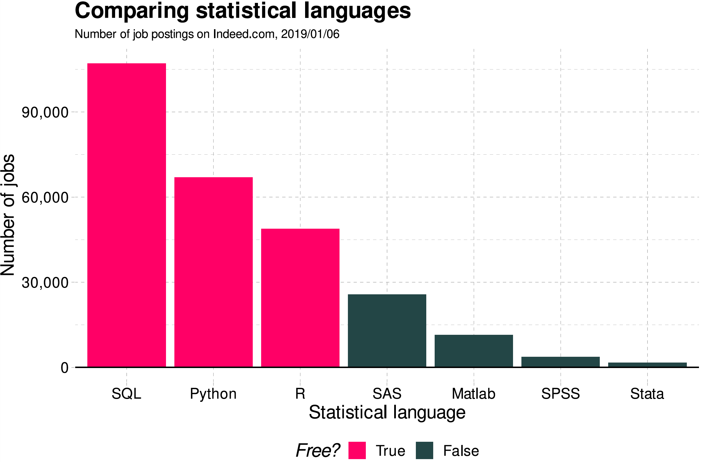
Why Python, R, and SQL?
For Your Information
Stack Overflow Trends
- We can see the trends of programming based on tags on the website, Stack Overflow
Getting started with pandas
pandas
![]()
pandasis a Python library including the following features:- Data manipulation and analysis,
- DataFrame objects and Series,
- Export and import data from files and web,
- Handling of missing data.
pandasprovides high-performance data structures and data analysis tools.
import pandas as pdGetting started with pandas
pd.DataFrame
DataFrameis the primary structure of pandas.DataFramerepresents a table of data with an ordered collection of columns.Each column can have a different data type.
DataFramecan be thought of as a dictionary ofSeriessharing the same index.
Getting started with pandas
Create DataFrame
pd.DataFrame()creates aDataFramewhich is a two-dimensional tabular-like structure with labeled axis (rows and columns).
data = {"state": ["Ohio", "Ohio", "Ohio", "Nevada", "Nevada", "Nevada"], "year": [2000, 2001, 2002, 2001, 2002, 2003], "population": [1.5, 1.7, 3.6, 2.4, 2.9, 3.2]}frame = pd.DataFrame(data)In this example the construction of the
DataFrameis done by passing a dictionary of equal-length lists.It is also possible to pass a dictionary of NumPy arrays.
- Passing a column that is not contained in the dict, it will be
marked with
NaN:
frame2 = pd.DataFrame(data, columns=["state", "year","population", "income"])frame2- The default index will be assigned automatically as with
Series.
- If we specify a sequence of columns, the DataFrame's columns will be arranged in that order:
frame2 = pd.DataFrame(data, columns=["year", "state", "population"])frame2We can pass the following types of objects to
pd.DataFrame():2D NumPy arrays
Dict of lists, tuples, dicts, arrays, or Series
List of lists, tuples, dicts, or Series
Another DataFrame
Getting started with pandas
Indexing DataFrame
- We can add a new column to
DataFrameas follows:
frame2["change"] = [1.2, -3.2, 0.4, -0.12, 2.4, 0.3]frame2["change"]- Selecting the column of
DataFrame, aSeriesis returned, - A attribute-like access, e.g.,
frame2.change, is also possible. - The returned
Serieshas the same index as the initialDataFrame.
- The result of using a list of multiple columns is a DataFrame:
frame2[ ["state", "population"] ]- We can name what the index and the columns are representing by using
index.nameandcolumns.namerespectively:
frame2.index.name = "number:"frame2.columns.name = "variable:"frame2- In
DataFrames, there is no default name for the index or the columns.
DataFrame.reindex()creates newDataFramewith data conformed to a new index, while the initialDataFramewill not be changed:
frame3 = frame.reindex([0, 2, 3, 4])frame3data = {"company": ["Daimler", "E.ON", "Siemens", "BASF", "BMW"],"price": [69.2, 8.11, 110.92, 87.28, 87.81],"volume": [4456290, 3667975, 3669487, 1778058, 1824582]}companies = pd.DataFrame(data)companiescompanies[2:]Index values that are not already present will be filled with
NaNby default.The
pd.isna()andpd.notna()functions detect missing data:
companies3 = companies.reindex(index = [0, 2, 3, 4, 5], columns=["company", "price", "market cap"])companies3pd.isna(companies3)pd.notna(companies3)- Calling
dropwith a sequence of labels will drop values from the row labels (axis 0):
obj = pd.Series(np.arange(5.), index = ["a", "b", "c", "d", "e"])objnew_obj = obj.drop("c")new_objobj.drop(["d", "c"])Getting started with pandas
Dropping columns
- With
DataFrame, index values can be deleted from either axis. To illustrate this, we first create an exampleDataFrame:
data = pd.DataFrame(np.arange(16).reshape((4, 4)), index = ["Ohio", "Colorado", "Utah", "New York"], columns=["one", "two", "three", "four"])datadata.drop(index = ["Colorado", "Ohio"])- To drop labels from the columns, we can use the
columnskeyword:
data.drop(columns=["two"])- We can also drop values from the columns by passing
axis=1oraxis="columns":
data.drop("two", axis=1)data.drop(["two", "four"], axis="columns")del DataFrame[column]deletes column fromDataFrame.
del data["two"]dataGetting started with pandas
Indexing, selecting and filtering
- Indexing of DataFrames works like indexing an
np.array.- We can use the default index values:
data = {"company": ["Daimler", "E.ON", "Siemens", "BASF", "BMW"],"price": [69.2, 8.11, 110.92, 87.28, 87.81],"volume": [4456290, 3667975, 3669487, 1778058, 1824582]}companies = pd.DataFrame(data)companiescompanies[2:]- We can also use a manually set index.
companies2 = pd.DataFrame(data, index = ["a", "b", "c", "d", "e"])companies2companies2["b":"d"]- When slicing with labels, the end element is inclusive.
DataFrame.loc()selects a subset of rows and columns from a DataFrame using axis labels.DataFrame.iloc()selects a subset of rows and columns from a DataFrame using integers.
companies2.loc[ "c", ["company", "price"] ]companies2.iloc[ 2, [0, 1] ]companies2.loc[ ["c", "d", "e"], ["volume", "price", "company"] ]companies2.iloc[ 2:, : :-1 ]df[val]selects single column or set of columns;
df.loc[val]selects single row or set of rows;df.loc[:, val]selects single column or set of columns;df.loc[val1, val2]selects row and column by label;
df.iloc[where]selects row or set of rows by integer position;df.iloc[:, where]selects column or set of columns by integer position;df.iloc[w1, w2]Select row and column by integer position.
Getting started with pandas
Operations between DataFrames and Series
- Here the
seriesis generated from the first row of theDataFrame:
companies3 = companies[["price", "volume"]]companies3.index = ["Daimler", "E.ON", "Siemens", "BASF", "BMW"]series = companies3.iloc[2]companies3series- By default, arithmetic operations between
DataFramesandSeriesmatch the index of theSerieson theDataFrame's columns:
companies3 + seriesDataFrame.add()does addition along a column matching theDataFrame's row index (axis=0).
series2 = companies3["price"]companies3.add(series2, axis=0)- Here are the example DataFrames to work with arithmetic operations:
df1 = pd.DataFrame( np.arange(9.).reshape((3, 3)), columns=list("bcd"), index = ["Ohio", "Texas", "Colorado"])df2 = pd.DataFrame( np.arange(12.).reshape((4, 3)), columns=list("bde"), index = ["Utah", "Ohio", "Texas", "Oregon"])df1df2df1 + df2DataFrame.Ttransposes DataFrame.
companies3.TGetting started with pandas
NumPy functions on DataFrame
DataFrame.apply(np.function, axis)applies a NumPy function on theDataFrameaxis.
companies3.apply(np.mean)companies3.apply(np.sqrt)companies3.apply(np.sqrt)[ :2]Getting started with pandas
Import/Export data
pd.read_csv("PATH_NAME_OF_*.csv") reads the csv file into DataFrame.
header=Nonedoes not read the top row of the csv file as column names.- We can set column names with
names, for example,names=["a", "b", "c", "d", "e"].
DataFrame.head()andDataFrame.tail()prints the first and last five rows on the Console, respectively.
nbc_show = pd.read_csv("https://bcdanl.github.io/data/nbc_show_na.csv")# `GRP`: audience size; `PE`: audience engagement.nbc_show.head() # showing the first five rowsnbc_show.tail() # showing the last five rowsGetting started with pandas
Export data
DataFrame.to_csv("filename") writes DataFrame to the csv file.
index = Falseandheader=Falsedo not write row index and column names in the csv file.- We can set column names with
header, for example,header=["a", "b", "c", "d", "e"].
nbc_show.to_csv("PATH_NAME_OF_THE_csv_FILE")Getting started with pandas
Summarizing DataFrame
DataFrame.count()returns a Series containing the number of non-missing values for each column.DataFrame.sum()returns a Series containing the sum of values for each column.DataFrame.mean()returns a Series containing the mean of values for each column.- Passing
axis="columns"oraxis=1sums across the columns instead:
- Passing
nbc_count = nbc_show.sum()nbc_sum = nbc_show.sum()nbc_sum_c = nbc_show.sum( axis="columns" )nbc_mean = nbc_show.mean()Getting started with pandas
Grouping DataFrame
DataFrame.groupby(col1, col2)groupsDataFrameby columns (grouping by one or more than two columns is also possible!).- Adding the functions
count(),sum(),mean()togroupby()returns the sum or the mean of the grouped columns.
- Adding the functions
nbc_genre_count = nbc_show.groupby(["Genre"]).count()nbc_genre_sum = nbc_show.groupby(["Genre"]).sum()nbc_network_genre_mean = nbc_show.groupby(["Network", "Genre"]).mean()Getting started with pandas
Sorting DataFrame
DataFrame.sort_index()sorts DataFrame by index on either axis.DataFrame.sort_index(axis="columns")sorts DataFrame by column index.DataFrame.sort_index(ascending=False)sorts DataFrame by either index in descending order.
nbc_show.sort_index()nbc_show.sort_index(ascending = False)nbc_show.sort_index(axis = "columns")nbc_show.sort_value()nbc_show.sort_value(ascending = False)nbc_show.sort_value(axis = "columns")Getting started with pandas
Sorting DataFrame
DataFrame.sort_value("SOME_VARIABLE")sorts DataFrame by values of SOME_VARIABLE.- For
Series.sort_value(), we do not need to provide"SOME_VARIABLE"in thesort_value()function.
- For
DataFrame.sort_value("SOME_VARIABLE", ascdening = False)sorts DataFrame by values of SOME_VARIABLE in descending order.
nbc_show.sort_value("GRP")nbc_show.sort_value("GRP", ascending = False)obj = pd.Series([4, np.nan, 7, np.nan, -3, 2])obj.sort_values()Getting started with pandas
Class Exercise
Use the nbc_show_na.csv file to answer the following questions:
Find the top show in terms of the value of
PEfor each Genre.Find the top show in terms of the value of
GRPfor each Network.Which genre does have the largest
GRPon average?
Workflow
Installing Python modules
- Let's install the Python visualization library
seaborn.
- Step 1. Open "Anaconda Prompt".
- Step 2. Type the following:
conda install seabornor
pip install seaborn- Step 1. Open "Terminal".
- Step 2. Type the following:
conda install seabornor
pip install seabornData Visualization with seaborn
Data Visualization
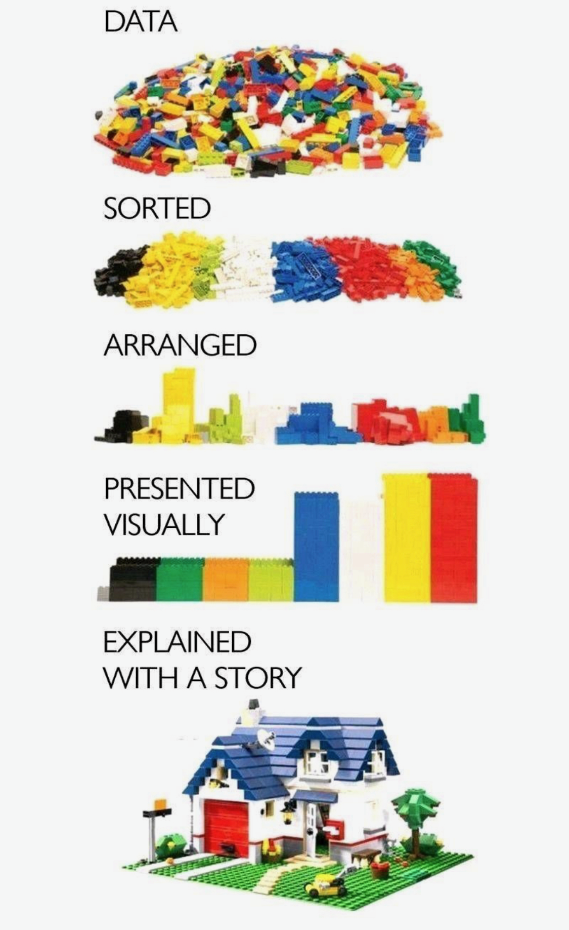
Graphs and charts let us explore and learn about the structure of the information we have in DataFrame.
Good data visualizations make it easier to communicate our ideas and findings to other people.
Exploratory Data Analysis (EDA)
We use visualization and summary statistics (e.g., mean, median, minimum, maximum) to explore our data in a systematic way.
EDA is an iterative cycle. We:
Generate questions about our data.
Search for answers by visualizing, transforming, and modelling our data.
Use what we learn to refine our questions and/or generate new questions.
seaborn
![]()
seabornis a Python data visualization library based onmatplotlib.- It allows us to easily create beautiful but complex graphics using a simple interface.
- It also provides a general improvement in the default appearance of
matplotlib-produced plots, and so I recommend using it by default.
import seaborn as snsData Visualization with seaborn
Types of plots
We will consider the following types of visualization:
Bar chart
Histogram
Scatter plot
Scatter plot with Fitted line
Line chart
Getting started with pandas
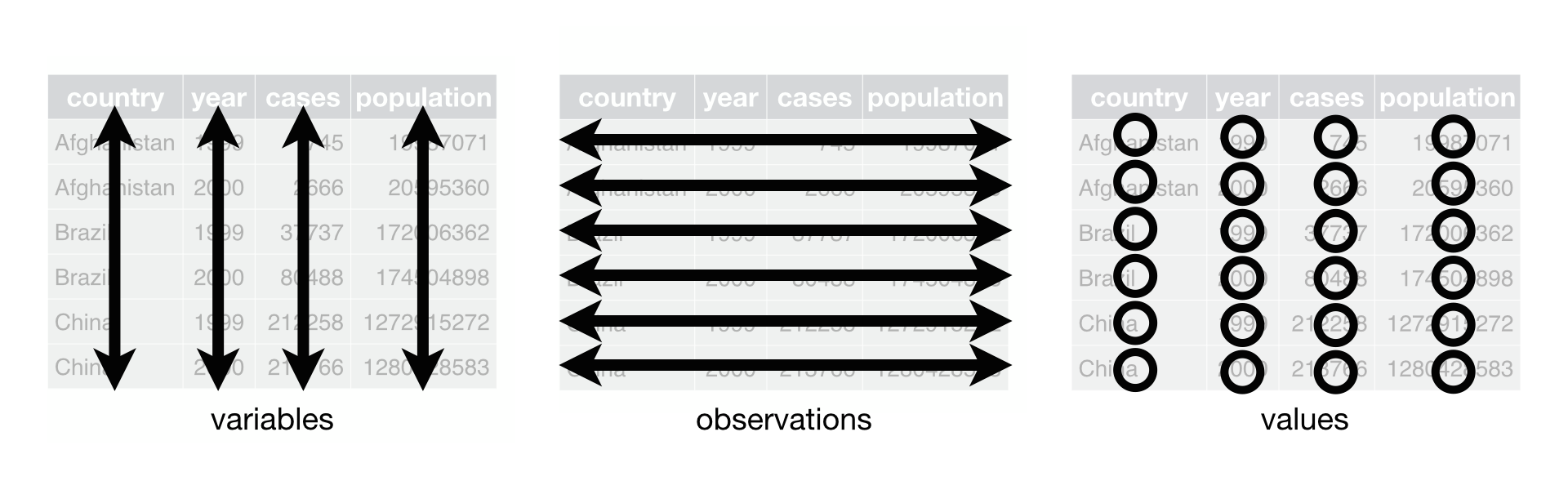
What is tidy DataFrame?
There are three rules which make a dataset tidy:
- Each variable has its own column.
- Each observation has its own row.
- Each value has its own cell.
Data Visualization with seaborn
Getting started with seaborn
- Let's get the names of
DataFrames provided by theseabornlibrary:
import seaborn as snsprint( sns.get_dataset_names() )- Let's use the
titanicandtipsDataFrames:
df_titanic = sns.load_dataset('titanic')df_titanic.head()df_tips = sns.load_dataset('tips')df_tips.head()Data Visualization with seaborn
Bar Chart
- A bar chart is used to plot the frequency of the different categories.
- It is useful to visualize how values of a categorical variable are distributed.
- A variable is categorical if it can only take one of a small set of values.
- We use
sns.countplot()function to plot a bar chart:
sns.countplot(x = 'sex', data = df_titanic)- Mapping
data: DataFrame.x: Name of a categorical variable (column) in DataFrame
Data Visualization with seaborn
Bar Chart
We can further break up the bars in the bar chart based on another categorical variable.
- This is useful to visualize the relationship between the two categorical variables.
sns.countplot(x = 'sex', hue = 'survived', data = df_titanic)- Mapping
hue: Name of a categorical variable
Data Visualization with seaborn
Histogram
- A histogram is a continuous version of a bar chart.
- It is used to plot the frequency of the different values.
- It is useful to visualize how values of a continuous variable are distributed.
- A variable is continuous if it can take any of an infinite set of ordered values.
- We use
sns.displot()function to plot a histogram:sns.displot(x = 'age',bins = 5 ,data = df_titanic)
- Mapping
bins: Number of bins
Data Visualization with seaborn
Scatter plot
A scatter plot is used to display the relationship between two continuous variables.
- We can see co-variation as a pattern in the scattered points.
We use
sns.scatterplot()function to plot a scatter plot:
sns.scatterplot(x = 'total_bill', y = 'tip', data = df_tips)- Mapping
x: Name of a continuous variable on the horizontal axisy: Name of a continuous variable on the vertical axis
Data Visualization with seaborn
Scatter plot
To the scatter plot, we can add a
hue-VARIABLEmapping to display how the relationship between two continuous variables varies byVARIABLE.Suppose we are interested in the following question:
- Q. Does a smoker and a non-smoker have a difference in tipping behavior?
sns.scatterplot(x = 'total_bill', y = 'tip', hue = 'smoker', data = df)Data Visualization with seaborn
Fitted line
From the scatter plot, it is often difficult to clearly see the relationship between two continuous variables.
sns.lmplot()adds a line that fits well into the scattered points.On average, the fitted line describes the relationship between two continuous variables.
sns.lmplot(x = 'total_bill', y = 'tip', data = df_tips)Data Visualization with seaborn
Scatter plot
To the scatter plot, we can add a
hue-VARIABLEmapping to display how the relationship between two continuous variables varies byVARIABLE.Using the fitted lines, let's answer the following question:
- Q. Does a smoker and a non-smoker have a difference in tipping behavior?
sns.scatterplot(x = 'total_bill', y = 'tip', hue = 'smoker', data = df_tips)Data Visualization with seaborn
Line cahrt
- A line chart is used to display the trend in a continuous variable or the change in a continuous variable over other variable.
- It draws a line by connecting the scattered points in order of the variable on the x-axis, so that it highlights exactly when changes occur.
- We use
sns.lineplot()function to plot a line plot:path_csv = '/Users/byeong-hakchoe/Google Drive/suny-geneseo/teaching-materials/lecture-data/dji.csv'dow = pd.read_csv(path_csv, index_col=0, parse_dates=True)sns.lineplot(x = 'Date',y = 'Close',data = dow)
- Mapping
x: Name of a continuous variable (often time variable) on the horizontal axisy: Name of a continuous variable on the vertical axis