Installing the Tools
RStudio Environment
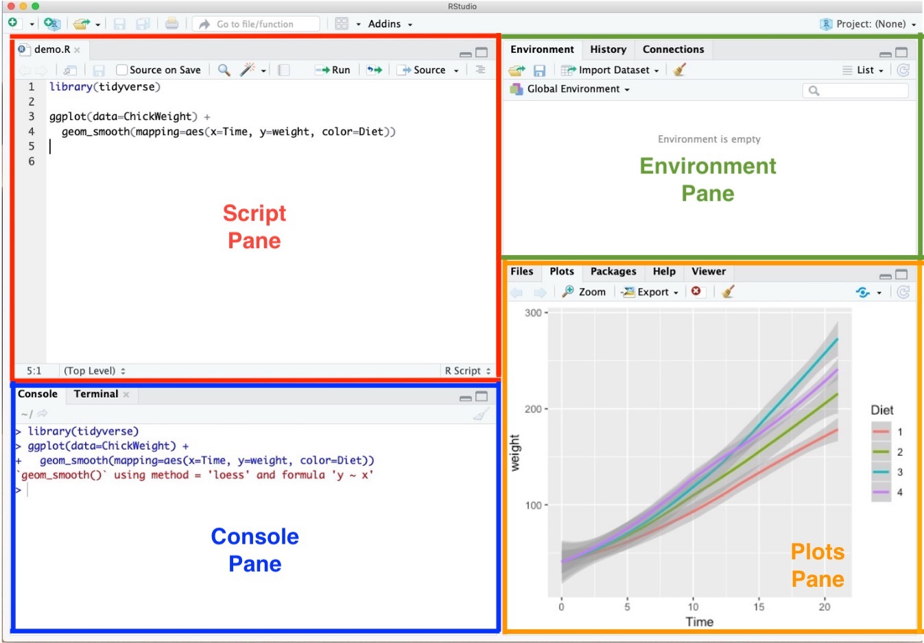
- Script Pane is where you write R commands in a script file that you can save.
- An R script is simply a text file containing R commands.
- RStudio will color-code different elements of your code to make it easier to read.
Installing the Tools
RStudio Environment
- Console Pane allows you to interact directly with the R interpreter and type commands where R will immediately execute them.
Installing the Tools
RStudio Environment
- Environment Pane is where you can see the values of variables, data frames, and other objects that are currently stored in memory.
Installing the Tools
RStudio Environment
- Plots Pane contains any graphics that you generate from your R code.
Workflow
- Home/End moves the blinking cursor bar to the beginning/End of the line.
- Ctrl (command for Mac Users) + / works too.
- Ctrl (command for Mac Users) + Z undoes the previous action.
- Ctrl (command for Mac Users) + Shift + Z redoes when undo is executed.
Ctrl (command for Mac Users) + F is useful when finding a phrase (and replace the phrase) in the RScript.
Auto-completion of command is useful.
- Type
librin the RScript in RStudio and wait for a second.
- Type
libr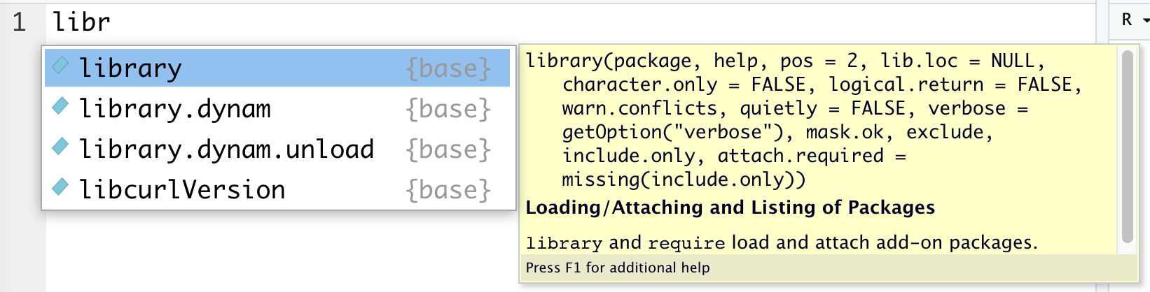
Workflow
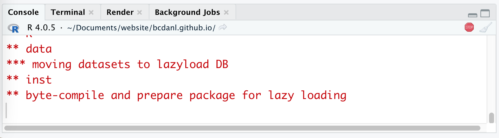
- To install R package
PACKAGE, useinstall.packages("PACKAGE").
install.packages("ggplot2") # installing package "ggplot2"- When the code is running, RStudio shows the STOP icon () at the top right corner in the Console Pane.
- Do not click it unless if you want to stop running the code.
Workflow
RStudio Options Setting

This option menu is found by menus as follows:
- Mac: RStudio > Preferences
- Windows: Tools > Global Options
Check as in the picture.
- Choose "Never" on "Save workplace to .RData on exit:".
Starting with R
R variables and data types
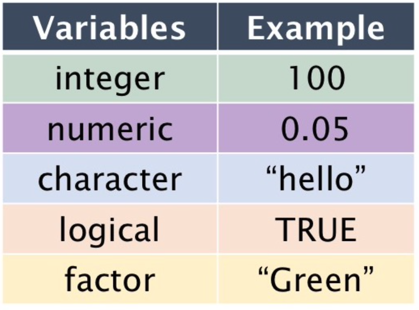
- Logical: TRUE or FALSE.
- Numeric: Decimal numbers
- Integer: Integers
- Character: Text strings
- Factor: Categorical values. Each possible value of a factor is known as a level.
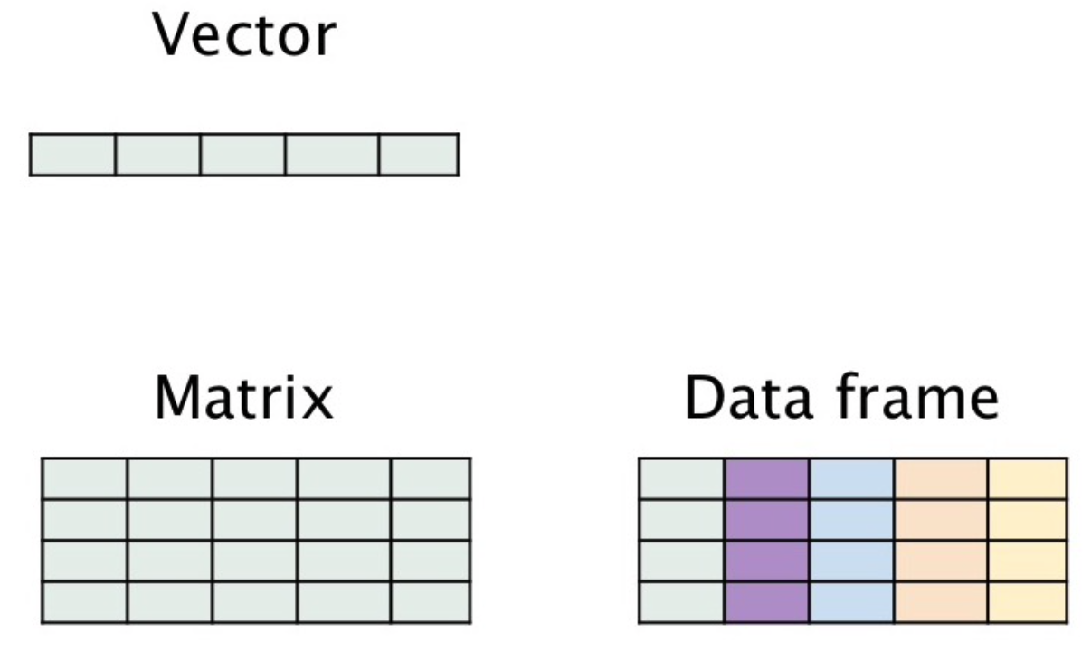
- vector: 1D collection of variables of the same type
- matrix: 2D collection of variables of the same type
- data.frame: 2D collection of variables of multiple types